> ## Documentation Index
> Fetch the complete documentation index at: https://aegean.ai/llms.txt
> Use this file to discover all available pages before exploring further.
# 3D Motion and Its 2D Projection
> How 3D motion of points and cameras projects to an image motion field, from vanishing points to the focus of expansion.
 *This section was written by [Kaushik Kachireddy](https://github.com/kaushik0x7d2) ([pull request #73](https://github.com/pantelis/eng-ai-agents/pull/73)), with help from an AI coding agent (Claude Code) on the code. It reproduces the ideas of Chapter 47 of [*Foundations of Computer Vision*](https://visionbook.mit.edu/2d_motion_from_3d.html) by Antonio Torralba, Phillip Isola, and William T. Freeman.*
When a 3D point moves, or the camera moves, how does its image on the camera plane move? This section answers that question with one long derivation: the **motion field equation** (47.8). Once you have it, every interesting motion phenomenon falls out as a special case: vanishing points, parallax, the focus of expansion, time-to-contact, and the way a zoom looks different from a dolly.
Each figure here is a diagram or a sketch of a vector field, drawn by encoding the underlying math in PyTorch. There are no photographs.
```python theme={null}
import torch
import matplotlib.pyplot as plt
from matplotlib.patches import Polygon, Rectangle, Circle, FancyArrowPatch, PathPatch
from matplotlib.path import Path
from mpl_toolkits.mplot3d import Axes3D # noqa: F401, registers 3d projection
torch.set_default_dtype(torch.float32)
_ = torch.manual_seed(0)
```
## Perspective projection of a moving point
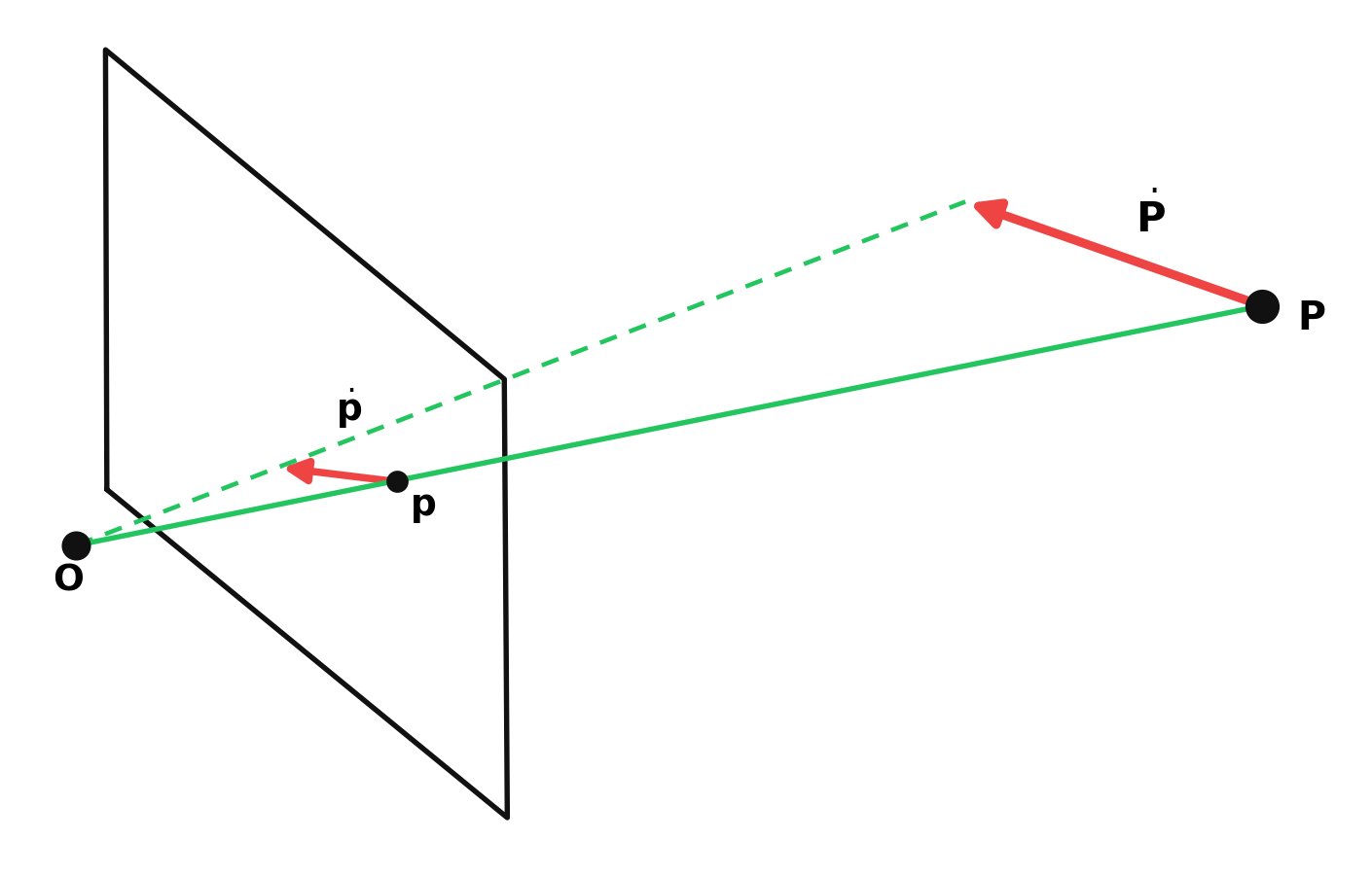
A 3D point $\mathbf{P} = (X, Y, Z)$ projects to image coordinates $\mathbf{p} = (x, y)$ through the pinhole camera with focal length $f$ (equation 47.9):
$x = f\,\frac{X}{Z}, \qquad y = f\,\frac{Y}{Z}.$
When $\mathbf{P}$ moves with velocity $\dot{\mathbf{P}} = (\dot X, \dot Y, \dot Z)$, the image point moves too. Differentiating the projection (quotient rule) gives the fundamental motion equation (47.1):
$\begin{bmatrix}\dot x\\\dot y\end{bmatrix} = \frac{1}{Z}\begin{bmatrix} f & 0 & -x \\ 0 & f & -y \end{bmatrix}\begin{bmatrix}\dot X\\\dot Y\\\dot Z\end{bmatrix}.$
The $1/Z$ factor is the entire reason vision can recover depth from motion, because closer points produce larger image-plane velocities than farther points moving the same way.
```python theme={null}
def project(P, f=1.0):
"""Pinhole projection (Eq. 47.9). P shape: (..., 3) → (..., 2)."""
X, Y, Z = P[..., 0], P[..., 1], P[..., 2]
return torch.stack([f * X / Z, f * Y / Z], dim=-1)
def project_velocity(P, P_dot, f=1.0):
"""Image-plane velocity from 3D point + 3D velocity (Eq. 47.1)."""
X, Y, Z = P[..., 0], P[..., 1], P[..., 2]
Xd, Yd, Zd = P_dot[..., 0], P_dot[..., 1], P_dot[..., 2]
x = f * X / Z
y = f * Y / Z
xd = (f * Xd - x * Zd) / Z
yd = (f * Yd - y * Zd) / Z
return torch.stack([xd, yd], dim=-1)
```
*This section was written by [Kaushik Kachireddy](https://github.com/kaushik0x7d2) ([pull request #73](https://github.com/pantelis/eng-ai-agents/pull/73)), with help from an AI coding agent (Claude Code) on the code. It reproduces the ideas of Chapter 47 of [*Foundations of Computer Vision*](https://visionbook.mit.edu/2d_motion_from_3d.html) by Antonio Torralba, Phillip Isola, and William T. Freeman.*
When a 3D point moves, or the camera moves, how does its image on the camera plane move? This section answers that question with one long derivation: the **motion field equation** (47.8). Once you have it, every interesting motion phenomenon falls out as a special case: vanishing points, parallax, the focus of expansion, time-to-contact, and the way a zoom looks different from a dolly.
Each figure here is a diagram or a sketch of a vector field, drawn by encoding the underlying math in PyTorch. There are no photographs.
```python theme={null}
import torch
import matplotlib.pyplot as plt
from matplotlib.patches import Polygon, Rectangle, Circle, FancyArrowPatch, PathPatch
from matplotlib.path import Path
from mpl_toolkits.mplot3d import Axes3D # noqa: F401, registers 3d projection
torch.set_default_dtype(torch.float32)
_ = torch.manual_seed(0)
```
## Perspective projection of a moving point
A 3D point $\mathbf{P} = (X, Y, Z)$ projects to image coordinates $\mathbf{p} = (x, y)$ through the pinhole camera with focal length $f$ (equation 47.9):
$x = f\,\frac{X}{Z}, \qquad y = f\,\frac{Y}{Z}.$
When $\mathbf{P}$ moves with velocity $\dot{\mathbf{P}} = (\dot X, \dot Y, \dot Z)$, the image point moves too. Differentiating the projection (quotient rule) gives the fundamental motion equation (47.1):
$\begin{bmatrix}\dot x\\\dot y\end{bmatrix} = \frac{1}{Z}\begin{bmatrix} f & 0 & -x \\ 0 & f & -y \end{bmatrix}\begin{bmatrix}\dot X\\\dot Y\\\dot Z\end{bmatrix}.$
The $1/Z$ factor is the entire reason vision can recover depth from motion, because closer points produce larger image-plane velocities than farther points moving the same way.
```python theme={null}
def project(P, f=1.0):
"""Pinhole projection (Eq. 47.9). P shape: (..., 3) → (..., 2)."""
X, Y, Z = P[..., 0], P[..., 1], P[..., 2]
return torch.stack([f * X / Z, f * Y / Z], dim=-1)
def project_velocity(P, P_dot, f=1.0):
"""Image-plane velocity from 3D point + 3D velocity (Eq. 47.1)."""
X, Y, Z = P[..., 0], P[..., 1], P[..., 2]
Xd, Yd, Zd = P_dot[..., 0], P_dot[..., 1], P_dot[..., 2]
x = f * X / Z
y = f * Y / Z
xd = (f * Xd - x * Zd) / Z
yd = (f * Yd - y * Zd) / Z
return torch.stack([xd, yd], dim=-1)
```
 ## Two easy cases of equation 47.1
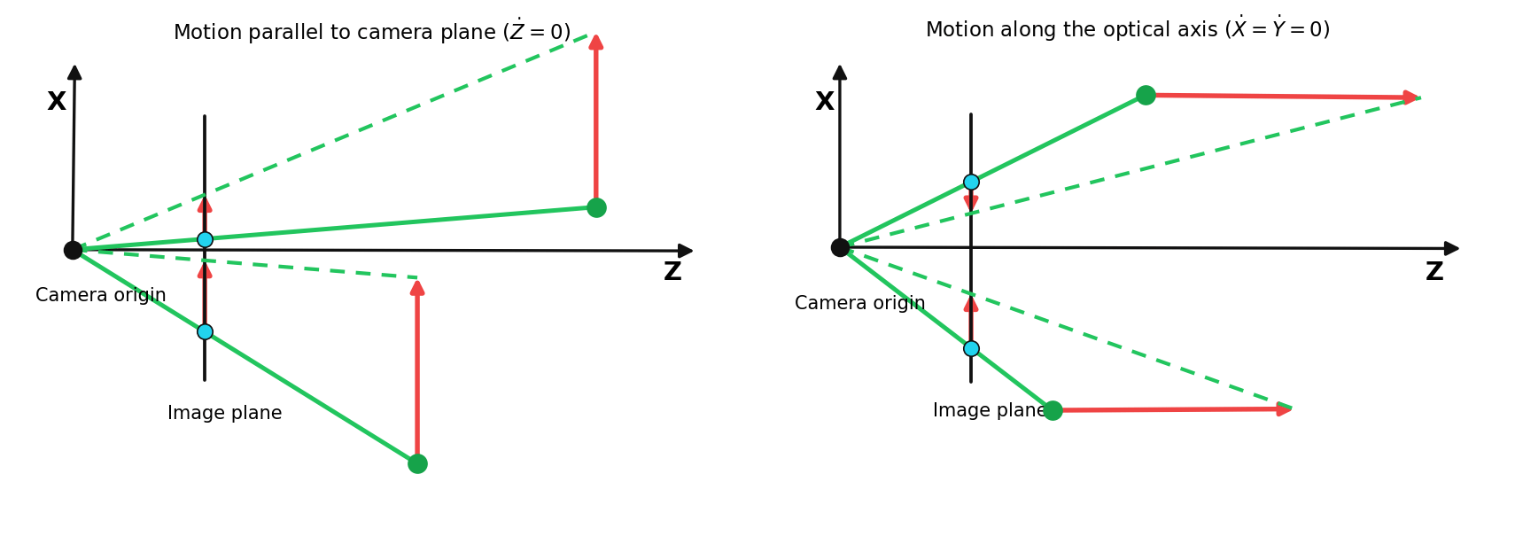
Equation 47.1 has three terms. Killing one at a time isolates the two simplest motion regimes:
**Motion parallel to the image plane** ($\dot Z = 0$, equation 47.2):
$\begin{bmatrix}\dot x\\\dot y\end{bmatrix} = \frac{f}{Z}\begin{bmatrix}\dot X\\\dot Y\end{bmatrix}.$
The magnitude is inversely proportional to depth: pure parallax.
**Motion along the optical axis** ($\dot X = \dot Y = 0$, equation 47.3):
$\begin{bmatrix}\dot x\\\dot y\end{bmatrix} = -\frac{\dot Z}{Z}\begin{bmatrix}x\\y\end{bmatrix}.$
Motion is radial, scaled by the ratio $\dot Z / Z$ (the **time-to-contact**).
Figure 47.2 sketches both.
## Two easy cases of equation 47.1
Equation 47.1 has three terms. Killing one at a time isolates the two simplest motion regimes:
**Motion parallel to the image plane** ($\dot Z = 0$, equation 47.2):
$\begin{bmatrix}\dot x\\\dot y\end{bmatrix} = \frac{f}{Z}\begin{bmatrix}\dot X\\\dot Y\end{bmatrix}.$
The magnitude is inversely proportional to depth: pure parallax.
**Motion along the optical axis** ($\dot X = \dot Y = 0$, equation 47.3):
$\begin{bmatrix}\dot x\\\dot y\end{bmatrix} = -\frac{\dot Z}{Z}\begin{bmatrix}x\\y\end{bmatrix}.$
Motion is radial, scaled by the ratio $\dot Z / Z$ (the **time-to-contact**).
Figure 47.2 sketches both.
 ## The vanishing point
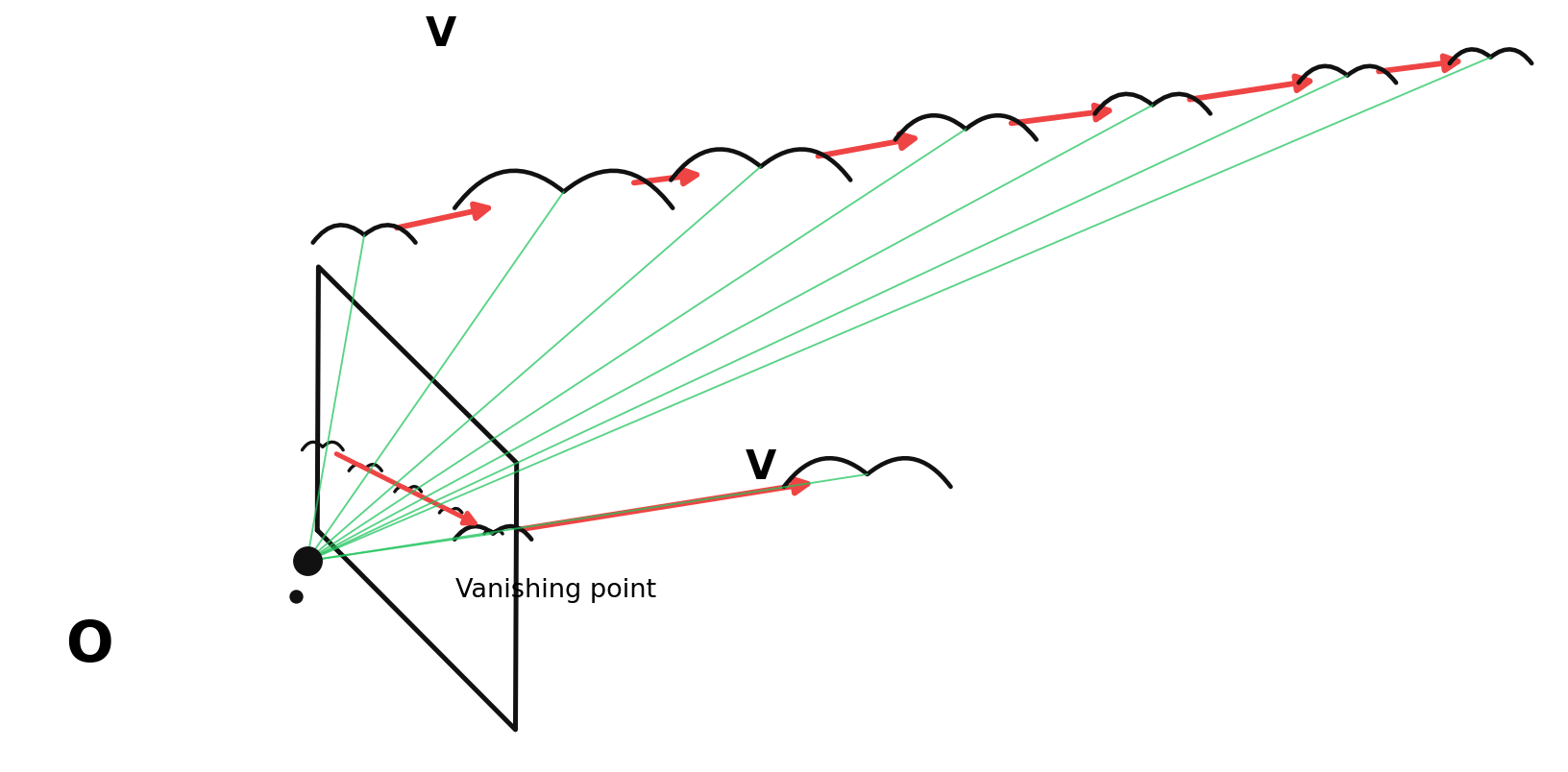
Let a point move with constant world velocity $\mathbf{V} = (V_X, V_Y, V_Z)$ from initial position $\mathbf{P}_0$. Its position is $\mathbf{P}(t) = \mathbf{P}_0 + t\mathbf{V}$, and its image is
$\mathbf{p}(t) = \frac{f}{P_{0,Z} + tV_Z}\begin{bmatrix}P_{0,X} + tV_X \\ P_{0,Y} + tV_Y\end{bmatrix}.$
As $t \to \infty$ the initial-position terms drop out and you land at the **vanishing point** (equation 47.4):
$x_{\infty} = f\,\frac{V_X}{V_Z},\qquad y_{\infty} = f\,\frac{V_Y}{V_Z}.$
The vanishing point depends only on the *direction* of motion, never on where the point started. Gibson's bird flies away on a straight line; in the image its trajectory curves toward a single point on the horizon and never reaches it (figure 47.3).
## The vanishing point
Let a point move with constant world velocity $\mathbf{V} = (V_X, V_Y, V_Z)$ from initial position $\mathbf{P}_0$. Its position is $\mathbf{P}(t) = \mathbf{P}_0 + t\mathbf{V}$, and its image is
$\mathbf{p}(t) = \frac{f}{P_{0,Z} + tV_Z}\begin{bmatrix}P_{0,X} + tV_X \\ P_{0,Y} + tV_Y\end{bmatrix}.$
As $t \to \infty$ the initial-position terms drop out and you land at the **vanishing point** (equation 47.4):
$x_{\infty} = f\,\frac{V_X}{V_Z},\qquad y_{\infty} = f\,\frac{V_Y}{V_Z}.$
The vanishing point depends only on the *direction* of motion, never on where the point started. Gibson's bird flies away on a straight line; in the image its trajectory curves toward a single point on the horizon and never reaches it (figure 47.3).
 ## The motion field under camera translation
When the *camera* translates with velocity $\mathbf{V}$ through a static world, each scene point moves with $-\mathbf{V}$ in the camera frame. Substituting $\dot{\mathbf{P}} = -\mathbf{V}$ into equation 47.1 gives the camera-translation motion field (equation 47.5):
$\begin{bmatrix}\dot x\\\dot y\end{bmatrix} = \frac{1}{Z}\begin{bmatrix}-f & 0 & x\\0 & -f & y\end{bmatrix}\begin{bmatrix}V_X\\V_Y\\V_Z\end{bmatrix}.$
The full motion field including rotation is given by equation 47.8, which the next cell encodes once and every later figure reuses.
```python theme={null}
def motion_field(x, y, Z, V, W, f=1.0):
"""Full image-plane motion field (Eq. 47.8).
Args:
x, y: image-plane coordinates, same shape.
Z: scene depth at each (x, y), broadcastable to x.
V: (3,) camera translational velocity (V_X, V_Y, V_Z).
W: (3,) camera angular velocity (W_X, W_Y, W_Z).
f: focal length.
Returns:
(xdot, ydot): same shape as x.
"""
Vx, Vy, Vz = V
Wx, Wy, Wz = W
trans_x = (-f * Vx + x * Vz) / Z
trans_y = (-f * Vy + y * Vz) / Z
rot_x = (x * y * Wx - (f * f + x * x) * Wy + f * y * Wz) / f
rot_y = ((f * f + y * y) * Wx - x * y * Wy - f * x * Wz) / f
return trans_x + rot_x, trans_y + rot_y
def image_grid(nx=15, ny=11, half_x=1.0, half_y=0.7):
"""A regular grid of image-plane sample points for quiver plots."""
xs = torch.linspace(-half_x, half_x, nx)
ys = torch.linspace(-half_y, half_y, ny)
gx, gy = torch.meshgrid(xs, ys, indexing="xy")
return gx, gy
```
### Lateral camera motion
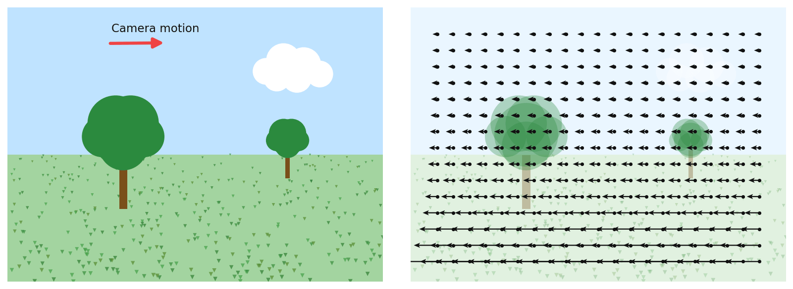
Driving past a roadside scene: $V_X \ne 0$, $V_Y = V_Z = 0$. The motion field collapses to
$\dot x = -\frac{f V_X}{Z}, \qquad \dot y = 0.$
Image-plane speed is inversely proportional to scene depth: close objects whip past while distant clouds barely move (figure 47.5).
## The motion field under camera translation
When the *camera* translates with velocity $\mathbf{V}$ through a static world, each scene point moves with $-\mathbf{V}$ in the camera frame. Substituting $\dot{\mathbf{P}} = -\mathbf{V}$ into equation 47.1 gives the camera-translation motion field (equation 47.5):
$\begin{bmatrix}\dot x\\\dot y\end{bmatrix} = \frac{1}{Z}\begin{bmatrix}-f & 0 & x\\0 & -f & y\end{bmatrix}\begin{bmatrix}V_X\\V_Y\\V_Z\end{bmatrix}.$
The full motion field including rotation is given by equation 47.8, which the next cell encodes once and every later figure reuses.
```python theme={null}
def motion_field(x, y, Z, V, W, f=1.0):
"""Full image-plane motion field (Eq. 47.8).
Args:
x, y: image-plane coordinates, same shape.
Z: scene depth at each (x, y), broadcastable to x.
V: (3,) camera translational velocity (V_X, V_Y, V_Z).
W: (3,) camera angular velocity (W_X, W_Y, W_Z).
f: focal length.
Returns:
(xdot, ydot): same shape as x.
"""
Vx, Vy, Vz = V
Wx, Wy, Wz = W
trans_x = (-f * Vx + x * Vz) / Z
trans_y = (-f * Vy + y * Vz) / Z
rot_x = (x * y * Wx - (f * f + x * x) * Wy + f * y * Wz) / f
rot_y = ((f * f + y * y) * Wx - x * y * Wy - f * x * Wz) / f
return trans_x + rot_x, trans_y + rot_y
def image_grid(nx=15, ny=11, half_x=1.0, half_y=0.7):
"""A regular grid of image-plane sample points for quiver plots."""
xs = torch.linspace(-half_x, half_x, nx)
ys = torch.linspace(-half_y, half_y, ny)
gx, gy = torch.meshgrid(xs, ys, indexing="xy")
return gx, gy
```
### Lateral camera motion
Driving past a roadside scene: $V_X \ne 0$, $V_Y = V_Z = 0$. The motion field collapses to
$\dot x = -\frac{f V_X}{Z}, \qquad \dot y = 0.$
Image-plane speed is inversely proportional to scene depth: close objects whip past while distant clouds barely move (figure 47.5).

 ### Forward camera motion and the focus of expansion
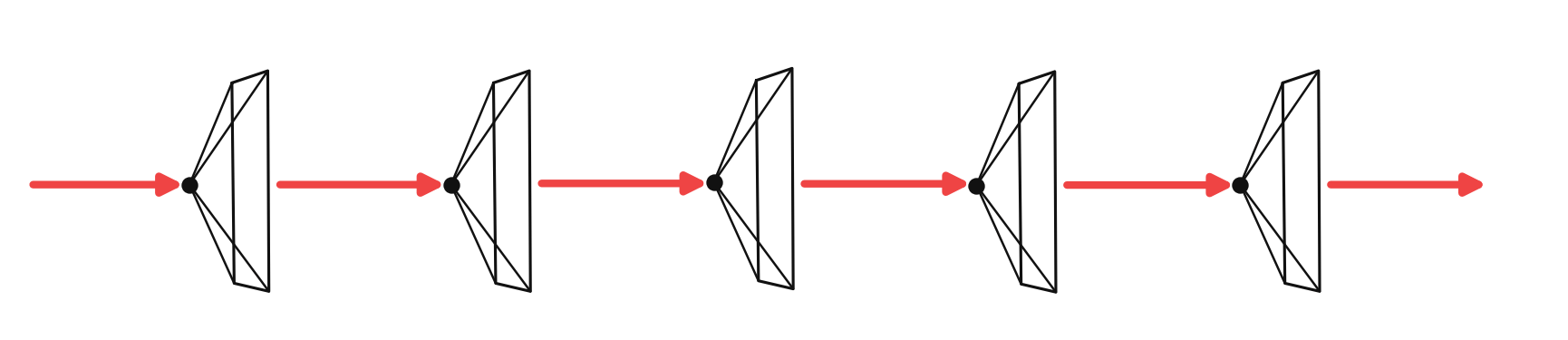
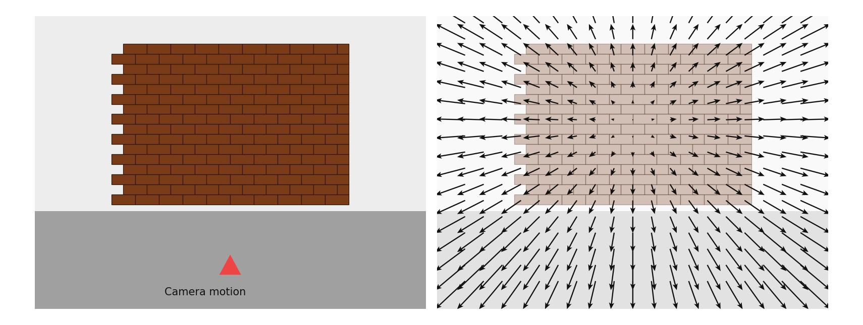
Driving toward a wall: $V_X = V_Y = 0$, $V_Z > 0$. Equation 47.5 simplifies to
$\dot x = \frac{V_Z}{Z}\,x, \qquad \dot y = \frac{V_Z}{Z}\,y,$
a radial flow centered at the origin. The point at which the field is zero is the **focus of expansion**, and the scaling factor $V_Z / Z$ is the inverse **time-to-contact**, the quantity a fly's-eye control loop reads off to time a landing.
### Forward camera motion and the focus of expansion
Driving toward a wall: $V_X = V_Y = 0$, $V_Z > 0$. Equation 47.5 simplifies to
$\dot x = \frac{V_Z}{Z}\,x, \qquad \dot y = \frac{V_Z}{Z}\,y,$
a radial flow centered at the origin. The point at which the field is zero is the **focus of expansion**, and the scaling factor $V_Z / Z$ is the inverse **time-to-contact**, the quantity a fly's-eye control loop reads off to time a landing.
 ## Camera rotation and the full motion field
Adding rotation, the point's velocity relative to a rotating camera with angular velocity $\mathbf{\Omega}$ is
$\dot{\mathbf{P}} = -\mathbf{V} - \mathbf{\Omega} \times \mathbf{P}.$
Plugging this into equation 47.1 produces the full motion field (equation 47.8):
$\begin{bmatrix}\dot x\\\dot y\end{bmatrix} = \underbrace{\frac{1}{Z}\begin{bmatrix}-f & 0 & x\\0 & -f & y\end{bmatrix}\begin{bmatrix}V_X\\V_Y\\V_Z\end{bmatrix}}_{\text{translation: depends on }Z} \;+\; \underbrace{\frac{1}{f}\begin{bmatrix}xy & -(f^2+x^2) & fy\\ f^2+y^2 & -xy & -fx\end{bmatrix}\begin{bmatrix}\Omega_X\\\Omega_Y\\\Omega_Z\end{bmatrix}}_{\text{rotation: independent of }Z}.$
Two qualitative consequences are worth noting:
* Rotational flow is **independent of depth**, so it tells you nothing about the scene's 3D structure.
* Translational flow scales as $1/Z$, so it carries all the depth information.
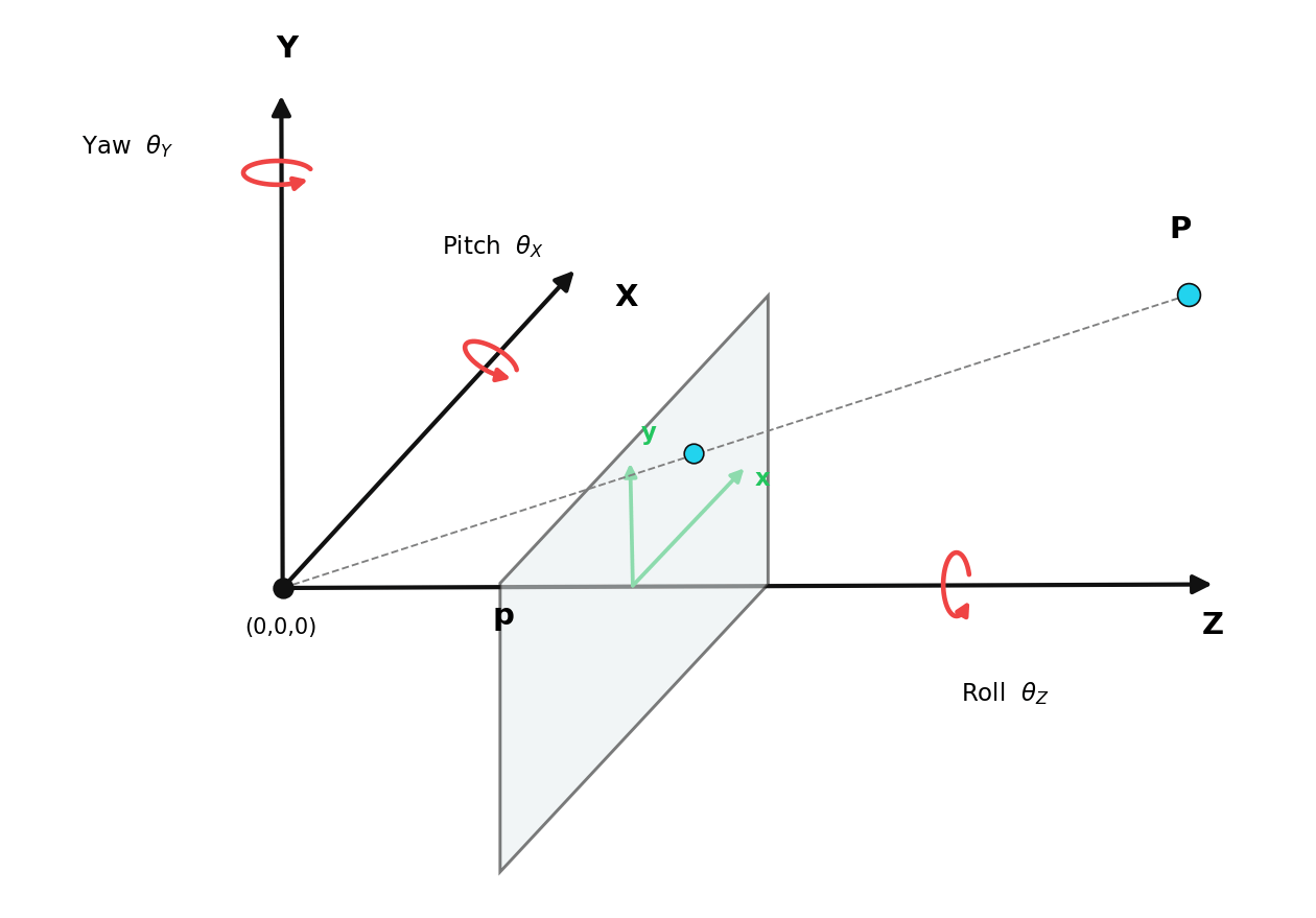
Figure 47.8 introduces the three rotation axes (yaw, pitch, roll) used throughout the rest of the chapter.
## Camera rotation and the full motion field
Adding rotation, the point's velocity relative to a rotating camera with angular velocity $\mathbf{\Omega}$ is
$\dot{\mathbf{P}} = -\mathbf{V} - \mathbf{\Omega} \times \mathbf{P}.$
Plugging this into equation 47.1 produces the full motion field (equation 47.8):
$\begin{bmatrix}\dot x\\\dot y\end{bmatrix} = \underbrace{\frac{1}{Z}\begin{bmatrix}-f & 0 & x\\0 & -f & y\end{bmatrix}\begin{bmatrix}V_X\\V_Y\\V_Z\end{bmatrix}}_{\text{translation: depends on }Z} \;+\; \underbrace{\frac{1}{f}\begin{bmatrix}xy & -(f^2+x^2) & fy\\ f^2+y^2 & -xy & -fx\end{bmatrix}\begin{bmatrix}\Omega_X\\\Omega_Y\\\Omega_Z\end{bmatrix}}_{\text{rotation: independent of }Z}.$
Two qualitative consequences are worth noting:
* Rotational flow is **independent of depth**, so it tells you nothing about the scene's 3D structure.
* Translational flow scales as $1/Z$, so it carries all the depth information.
Figure 47.8 introduces the three rotation axes (yaw, pitch, roll) used throughout the rest of the chapter.
 ### Rotation around the optical axis ($\Omega_X = \Omega_Y = 0$)
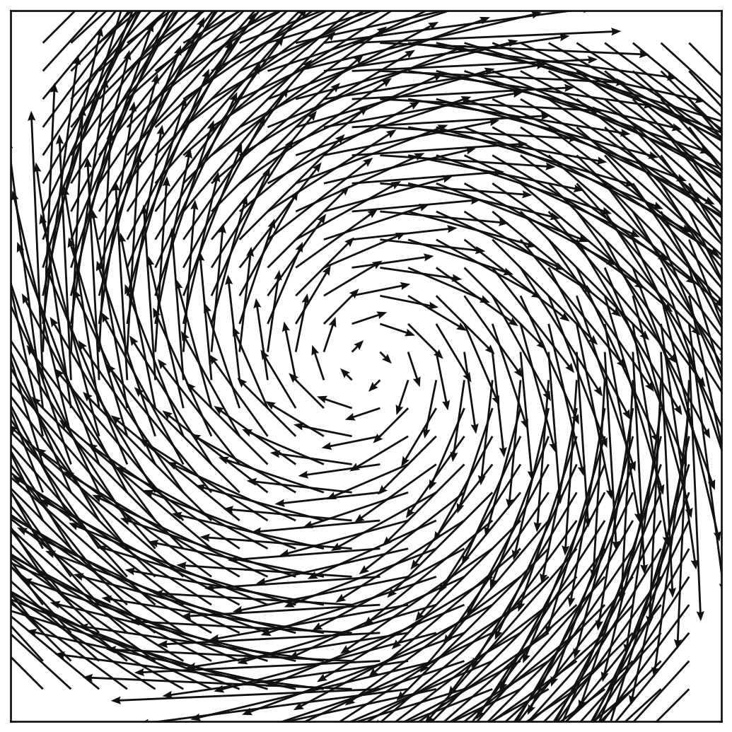
With only $\Omega_Z$ active, equation 47.8 collapses to
$\dot x = \Omega_Z\,y,\qquad \dot y = -\Omega_Z\,x,$
the velocity field of rigid rotation about the image origin. Every concentric circle is an integral curve (figure 47.9).
### Rotation around the optical axis ($\Omega_X = \Omega_Y = 0$)
With only $\Omega_Z$ active, equation 47.8 collapses to
$\dot x = \Omega_Z\,y,\qquad \dot y = -\Omega_Z\,x,$
the velocity field of rigid rotation about the image origin. Every concentric circle is an integral curve (figure 47.9).
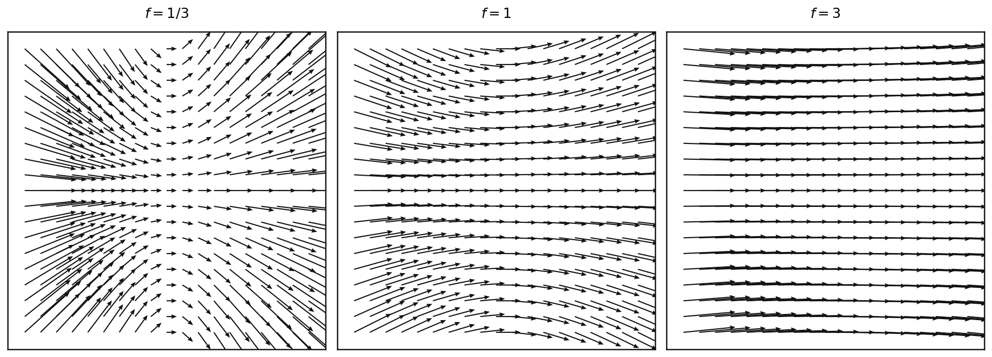
 ## Rotation under varying focal length
Y-axis rotation with $\Omega_X = \Omega_Z = 0$ produces
$\dot x = -\frac{(f^2 + x^2)}{f}\,\Omega_Y,\qquad \dot y = -\frac{xy}{f}\,\Omega_Y,$
which depends strongly on $f$. Wide-angle lenses ($f$ small) produce flows with sharp curvature near the edges; long lenses ($f$ large) produce nearly uniform horizontal flow. Figure 47.10 sweeps $f \in \{1/3, 1, 3\}$ with the same scene and angular velocity.
## Rotation under varying focal length
Y-axis rotation with $\Omega_X = \Omega_Z = 0$ produces
$\dot x = -\frac{(f^2 + x^2)}{f}\,\Omega_Y,\qquad \dot y = -\frac{xy}{f}\,\Omega_Y,$
which depends strongly on $f$. Wide-angle lenses ($f$ small) produce flows with sharp curvature near the edges; long lenses ($f$ large) produce nearly uniform horizontal flow. Figure 47.10 sweeps $f \in \{1/3, 1, 3\}$ with the same scene and angular velocity.
 ## Concluding remarks
The whole chapter rests on three ideas:
1. **Differentiate the projection** $\mathbf{p} = (fX/Z, fY/Z)$ to get the image-plane motion of any moving 3D point (eq. 47.1).
2. **Substitute the camera's rigid-body kinematics** $\dot{\mathbf{P}} = -\mathbf{V} - \mathbf{\Omega}\times\mathbf{P}$ to get the motion field (eq. 47.8).
3. **Read off special cases**: vanishing points (47.4), depth-modulated parallax (47.5), focus of expansion and time-to-contact (47.6), depth-independent rotation (47.7), focal-length sensitivity (47.10).
The next chapter of the book (48, optical flow) flips the script: given two frames, *recover* the motion field. The geometry here is the forward model that chapter inverts.
***
[Edit this page on GitHub](https://github.com/aegean-ai/eaia/edit/main/src/aiml-common/lectures/3d-reconstruction/3d-motion-projection/index.mdx) or [file an issue](https://github.com/aegean-ai/eaia/issues/new/choose).
## Concluding remarks
The whole chapter rests on three ideas:
1. **Differentiate the projection** $\mathbf{p} = (fX/Z, fY/Z)$ to get the image-plane motion of any moving 3D point (eq. 47.1).
2. **Substitute the camera's rigid-body kinematics** $\dot{\mathbf{P}} = -\mathbf{V} - \mathbf{\Omega}\times\mathbf{P}$ to get the motion field (eq. 47.8).
3. **Read off special cases**: vanishing points (47.4), depth-modulated parallax (47.5), focus of expansion and time-to-contact (47.6), depth-independent rotation (47.7), focal-length sensitivity (47.10).
The next chapter of the book (48, optical flow) flips the script: given two frames, *recover* the motion field. The geometry here is the forward model that chapter inverts.
***
[Edit this page on GitHub](https://github.com/aegean-ai/eaia/edit/main/src/aiml-common/lectures/3d-reconstruction/3d-motion-projection/index.mdx) or [file an issue](https://github.com/aegean-ai/eaia/issues/new/choose).