> ## Documentation Index
> Fetch the complete documentation index at: https://aegean.ai/llms.txt
> Use this file to discover all available pages before exploring further.
# Representing Images and Geometry
> Homogeneous coordinates, 2D image transformations, point and line duality, image warping, and implicit image representations.
 *This section was written by [Kaushik Kachireddy](https://github.com/kaushik0x7d2) ([pull request #74](https://github.com/pantelis/eng-ai-agents/pull/74)), with help from an AI coding agent (Claude Code) on the code. It reproduces the ideas of Chapter 38 of [*Foundations of Computer Vision*](https://visionbook.mit.edu/homogeneous_coordinates.html) by Antonio Torralba, Phillip Isola, and William T. Freeman.*
This section lays the foundation for all the geometry that follows. Three ideas drive it:
1. **Homogeneous coordinates** let you write translation, rotation, scaling, shearing, and projective warps as a single matrix multiplication.
2. **Lines and points are dual** under the cross product in homogeneous form: joining two points and intersecting two lines are the same operation.
3. **Implicit image representations** (SIREN-style networks that map $(x,y)\to \text{intensity}$) give you sub-pixel image access without an interpolation kernel, so geometric transformations become inverse-coordinate evaluations.
The figures are regenerated in PyTorch. Two of them go furthest: figure 38.8 reframes warping as a 1D convolution on coordinates, and figure 38.12 replaces the pixel grid with a neural network.
```python theme={null}
import math
from pathlib import Path
import torch
import torch.nn as nn
import kornia.geometry.transform as KT
import matplotlib.pyplot as plt
from matplotlib.patches import Polygon, Rectangle, Circle, FancyArrowPatch, PathPatch
from matplotlib.path import Path as MplPath
from matplotlib.collections import LineCollection
from mpl_toolkits.mplot3d.art3d import Poly3DCollection
from PIL import Image, ImageDraw
import skimage.data
torch.set_default_dtype(torch.float32)
_ = torch.manual_seed(0)
```
## Homogeneous and heterogeneous coordinates
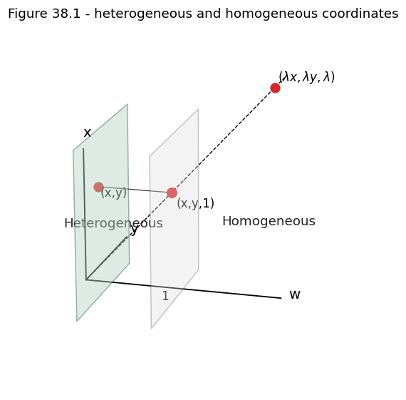
Heterogeneous coordinates write a 2D point as $(x, y)$. Homogeneous coordinates write the same point as $(x, y, 1)$, and also as $(\lambda x, \lambda y, \lambda)$ for any $\lambda \ne 0$. All points on the ray through the origin and $(x, y, 1)$ represent the same 2D point. Converting back means dividing by $w$:
$\begin{bmatrix}x\\y\\w\end{bmatrix} \;\longrightarrow\; \left(\frac{x}{w}, \frac{y}{w}\right).$
The payoff is that translation, an *addition* in heterogeneous coordinates, becomes a *multiplication* in homogeneous coordinates. This uniformity lets you compose any sequence of geometric transformations into a single matrix product.
```python theme={null}
def to_homogeneous(p):
"""Append a 1 to the last axis. (..., D) -> (..., D+1)."""
return torch.cat([p, torch.ones_like(p[..., :1])], dim=-1)
def from_homogeneous(p):
"""Divide by last coord. (..., D+1) -> (..., D)."""
return p[..., :-1] / p[..., -1:]
```
*This section was written by [Kaushik Kachireddy](https://github.com/kaushik0x7d2) ([pull request #74](https://github.com/pantelis/eng-ai-agents/pull/74)), with help from an AI coding agent (Claude Code) on the code. It reproduces the ideas of Chapter 38 of [*Foundations of Computer Vision*](https://visionbook.mit.edu/homogeneous_coordinates.html) by Antonio Torralba, Phillip Isola, and William T. Freeman.*
This section lays the foundation for all the geometry that follows. Three ideas drive it:
1. **Homogeneous coordinates** let you write translation, rotation, scaling, shearing, and projective warps as a single matrix multiplication.
2. **Lines and points are dual** under the cross product in homogeneous form: joining two points and intersecting two lines are the same operation.
3. **Implicit image representations** (SIREN-style networks that map $(x,y)\to \text{intensity}$) give you sub-pixel image access without an interpolation kernel, so geometric transformations become inverse-coordinate evaluations.
The figures are regenerated in PyTorch. Two of them go furthest: figure 38.8 reframes warping as a 1D convolution on coordinates, and figure 38.12 replaces the pixel grid with a neural network.
```python theme={null}
import math
from pathlib import Path
import torch
import torch.nn as nn
import kornia.geometry.transform as KT
import matplotlib.pyplot as plt
from matplotlib.patches import Polygon, Rectangle, Circle, FancyArrowPatch, PathPatch
from matplotlib.path import Path as MplPath
from matplotlib.collections import LineCollection
from mpl_toolkits.mplot3d.art3d import Poly3DCollection
from PIL import Image, ImageDraw
import skimage.data
torch.set_default_dtype(torch.float32)
_ = torch.manual_seed(0)
```
## Homogeneous and heterogeneous coordinates
Heterogeneous coordinates write a 2D point as $(x, y)$. Homogeneous coordinates write the same point as $(x, y, 1)$, and also as $(\lambda x, \lambda y, \lambda)$ for any $\lambda \ne 0$. All points on the ray through the origin and $(x, y, 1)$ represent the same 2D point. Converting back means dividing by $w$:
$\begin{bmatrix}x\\y\\w\end{bmatrix} \;\longrightarrow\; \left(\frac{x}{w}, \frac{y}{w}\right).$
The payoff is that translation, an *addition* in heterogeneous coordinates, becomes a *multiplication* in homogeneous coordinates. This uniformity lets you compose any sequence of geometric transformations into a single matrix product.
```python theme={null}
def to_homogeneous(p):
"""Append a 1 to the last axis. (..., D) -> (..., D+1)."""
return torch.cat([p, torch.ones_like(p[..., :1])], dim=-1)
def from_homogeneous(p):
"""Divide by last coord. (..., D+1) -> (..., D)."""
return p[..., :-1] / p[..., -1:]
```
 ## 2D image transformations
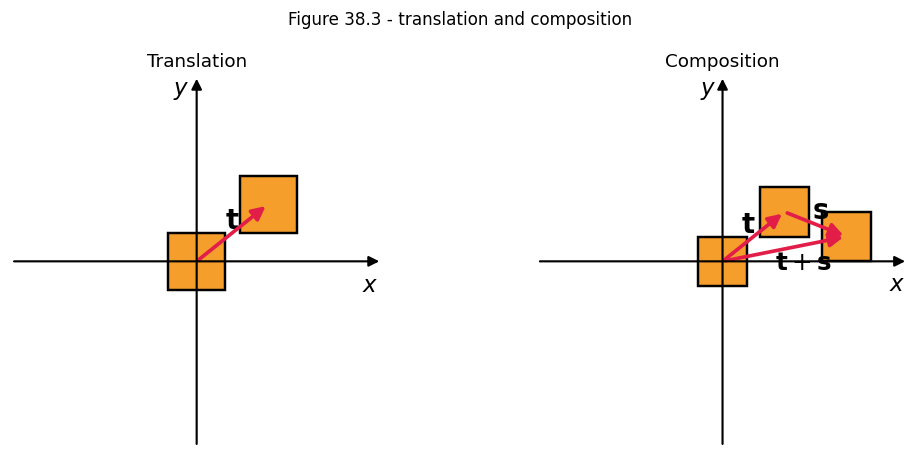
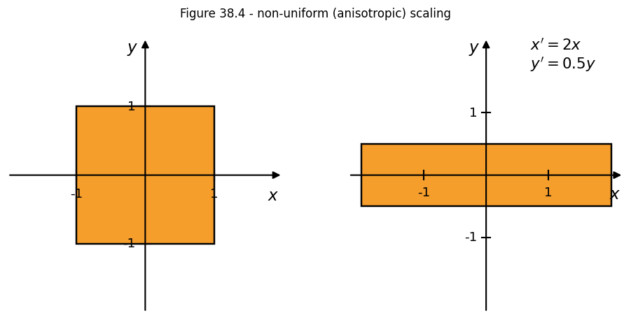
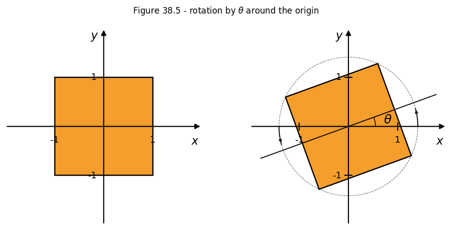
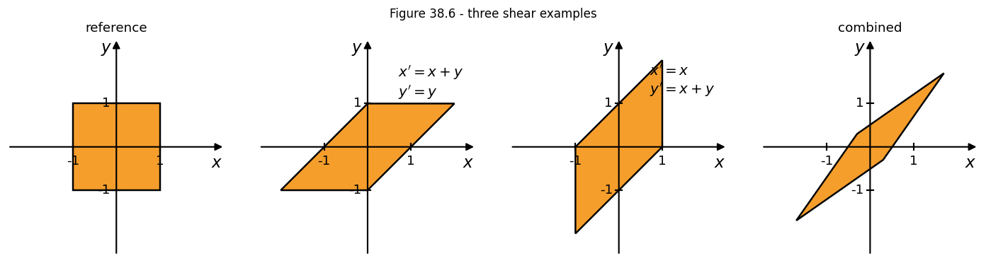
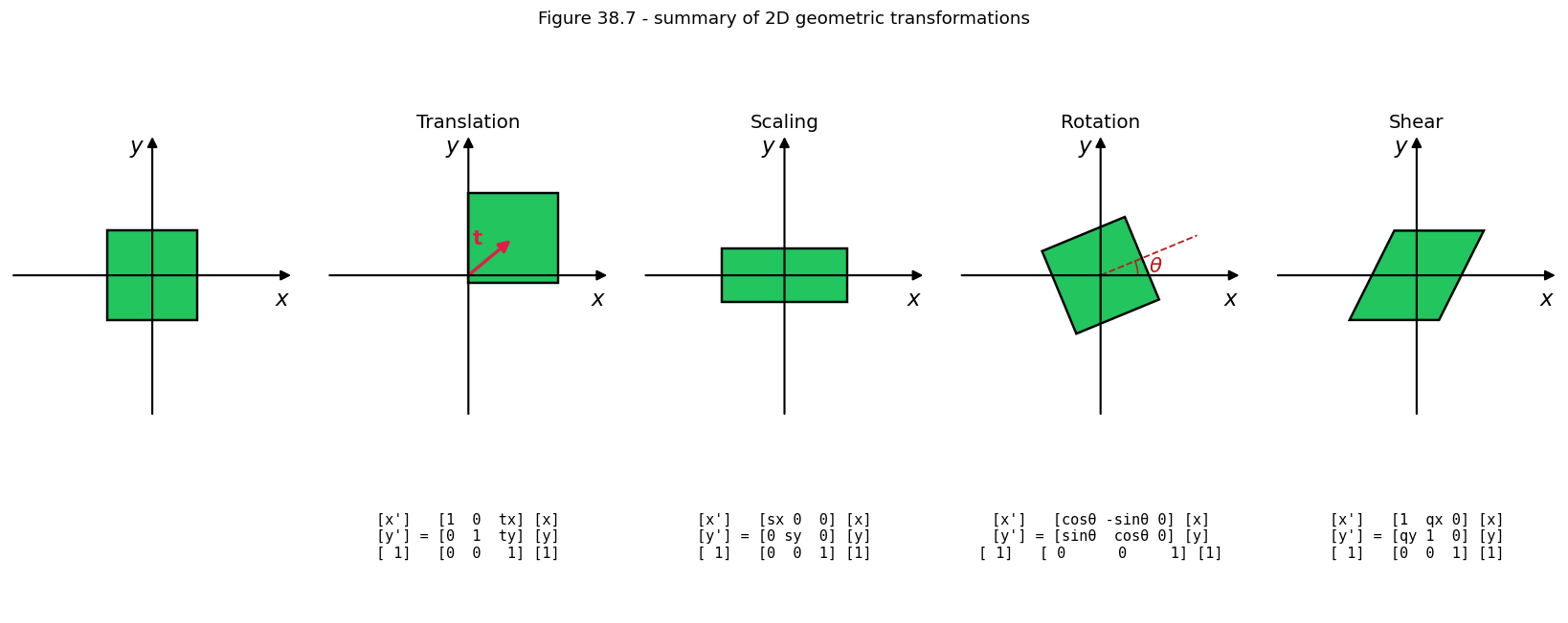
Every transformation that follows is a $3\times 3$ matrix acting on homogeneous points. The book applies each transformation to a photograph of a clock. Here a wall-clock image stands in for it, and each matrix is applied as an actual image warp with `kornia.geometry.transform.warp_affine`, so what you see is the matrix acting on real pixels.
```python theme={null}
# Reference object: an AI-generated wall-clock image supplied by the contributor,
# loaded as a torch tensor. It stands in for the book's own clock photograph,
# which is not reproduced here.
def apply_T(M, pts):
"""Apply 3x3 homogeneous matrix to (N, 2) points - still used by the
hand-written forward_warp / backward_warp helpers in the warping section."""
return from_homogeneous(to_homogeneous(pts) @ M.T)
CLOCK_URL = ("https://raw.githubusercontent.com/pantelis/eng-ai-agents/main/notebooks/CV/"
"mit-foundations/chapter-38-images-and-geometry/assets/wallclock.png")
def clock_path():
# Find the clock image next to this section, or download it once.
for candidate in (Path("assets"), Path("notebooks/CV/mit-foundations/chapter-38-images-and-geometry/assets")):
if (candidate / "wallclock.png").exists():
return candidate / "wallclock.png"
import urllib.request
local = Path("wallclock.png")
if not local.exists():
urllib.request.urlretrieve(CLOCK_URL, local)
return local
def render_clock(size=256):
"""Load the bundled wall-clock asset (assets/wallclock.png) as-is.
The asset already has natural background padding around the clock, so we
just resize to `size` if needed and return the tensor unchanged."""
img = Image.open(clock_path()).convert("L")
if img.size != (size, size):
img = img.resize((size, size), Image.LANCZOS)
pixels = torch.frombuffer(bytearray(img.tobytes()), dtype=torch.uint8)
return pixels.to(torch.float32).view(size, size) / 255.0
CLOCK = render_clock(256)
CLOCK_H, CLOCK_W = CLOCK.shape
def warp_image(img, M_3x3, dsize=None):
"""Apply a 3x3 homogeneous matrix to an image via kornia (backward, bilinear).
Convention: M maps source pixel coords to target coords."""
H, W = img.shape
if dsize is None:
dsize = (H, W)
img_bchw = img.unsqueeze(0).unsqueeze(0)
M_b23 = M_3x3[:2, :3].unsqueeze(0)
out = KT.warp_affine(img_bchw, M_b23, dsize=dsize, mode="bilinear", padding_mode="border")
return out.squeeze(0).squeeze(0)
```
```python theme={null}
def T_translate(tx, ty):
return torch.tensor([[1.0, 0.0, tx], [0.0, 1.0, ty], [0.0, 0.0, 1.0]])
def T_scale(sx, sy, cx=0.0, cy=0.0):
"""Scale about the point (cx, cy)."""
return (
torch.tensor([[1.0, 0.0, cx], [0.0, 1.0, cy], [0.0, 0.0, 1.0]])
@ torch.tensor([[sx, 0.0, 0.0], [0.0, sy, 0.0], [0.0, 0.0, 1.0]])
@ torch.tensor([[1.0, 0.0, -cx], [0.0, 1.0, -cy], [0.0, 0.0, 1.0]])
)
def T_rotate(theta, cx=0.0, cy=0.0):
"""Rotation about (cx, cy) by theta radians (image-down y)."""
c, s = math.cos(theta), math.sin(theta)
return (
torch.tensor([[1.0, 0.0, cx], [0.0, 1.0, cy], [0.0, 0.0, 1.0]])
@ torch.tensor([[c, -s, 0.0], [s, c, 0.0], [0.0, 0.0, 1.0]])
@ torch.tensor([[1.0, 0.0, -cx], [0.0, 1.0, -cy], [0.0, 0.0, 1.0]])
)
def T_shear(shx, shy):
return torch.tensor([[1.0, shx, 0.0], [shy, 1.0, 0.0], [0.0, 0.0, 1.0]])
def T_projective_warp(strength=0.0028):
"""A homography that visibly tilts the image (right side closer to camera).
Bigger strength -> more pronounced trapezoidal warp."""
M = torch.eye(3)
M[2, 0] = strength # right side shrinks toward vanishing point
M[2, 1] = -strength * 0.55 # top tilts inward
return M
# Inverse of each transform is what warp_affine wants (backward mapping),
# but kornia's warp_affine expects the source-to-target matrix and inverts
# internally, so the forward transform is passed.
cx, cy = CLOCK_W / 2, CLOCK_H / 2
```
## 2D image transformations
Every transformation that follows is a $3\times 3$ matrix acting on homogeneous points. The book applies each transformation to a photograph of a clock. Here a wall-clock image stands in for it, and each matrix is applied as an actual image warp with `kornia.geometry.transform.warp_affine`, so what you see is the matrix acting on real pixels.
```python theme={null}
# Reference object: an AI-generated wall-clock image supplied by the contributor,
# loaded as a torch tensor. It stands in for the book's own clock photograph,
# which is not reproduced here.
def apply_T(M, pts):
"""Apply 3x3 homogeneous matrix to (N, 2) points - still used by the
hand-written forward_warp / backward_warp helpers in the warping section."""
return from_homogeneous(to_homogeneous(pts) @ M.T)
CLOCK_URL = ("https://raw.githubusercontent.com/pantelis/eng-ai-agents/main/notebooks/CV/"
"mit-foundations/chapter-38-images-and-geometry/assets/wallclock.png")
def clock_path():
# Find the clock image next to this section, or download it once.
for candidate in (Path("assets"), Path("notebooks/CV/mit-foundations/chapter-38-images-and-geometry/assets")):
if (candidate / "wallclock.png").exists():
return candidate / "wallclock.png"
import urllib.request
local = Path("wallclock.png")
if not local.exists():
urllib.request.urlretrieve(CLOCK_URL, local)
return local
def render_clock(size=256):
"""Load the bundled wall-clock asset (assets/wallclock.png) as-is.
The asset already has natural background padding around the clock, so we
just resize to `size` if needed and return the tensor unchanged."""
img = Image.open(clock_path()).convert("L")
if img.size != (size, size):
img = img.resize((size, size), Image.LANCZOS)
pixels = torch.frombuffer(bytearray(img.tobytes()), dtype=torch.uint8)
return pixels.to(torch.float32).view(size, size) / 255.0
CLOCK = render_clock(256)
CLOCK_H, CLOCK_W = CLOCK.shape
def warp_image(img, M_3x3, dsize=None):
"""Apply a 3x3 homogeneous matrix to an image via kornia (backward, bilinear).
Convention: M maps source pixel coords to target coords."""
H, W = img.shape
if dsize is None:
dsize = (H, W)
img_bchw = img.unsqueeze(0).unsqueeze(0)
M_b23 = M_3x3[:2, :3].unsqueeze(0)
out = KT.warp_affine(img_bchw, M_b23, dsize=dsize, mode="bilinear", padding_mode="border")
return out.squeeze(0).squeeze(0)
```
```python theme={null}
def T_translate(tx, ty):
return torch.tensor([[1.0, 0.0, tx], [0.0, 1.0, ty], [0.0, 0.0, 1.0]])
def T_scale(sx, sy, cx=0.0, cy=0.0):
"""Scale about the point (cx, cy)."""
return (
torch.tensor([[1.0, 0.0, cx], [0.0, 1.0, cy], [0.0, 0.0, 1.0]])
@ torch.tensor([[sx, 0.0, 0.0], [0.0, sy, 0.0], [0.0, 0.0, 1.0]])
@ torch.tensor([[1.0, 0.0, -cx], [0.0, 1.0, -cy], [0.0, 0.0, 1.0]])
)
def T_rotate(theta, cx=0.0, cy=0.0):
"""Rotation about (cx, cy) by theta radians (image-down y)."""
c, s = math.cos(theta), math.sin(theta)
return (
torch.tensor([[1.0, 0.0, cx], [0.0, 1.0, cy], [0.0, 0.0, 1.0]])
@ torch.tensor([[c, -s, 0.0], [s, c, 0.0], [0.0, 0.0, 1.0]])
@ torch.tensor([[1.0, 0.0, -cx], [0.0, 1.0, -cy], [0.0, 0.0, 1.0]])
)
def T_shear(shx, shy):
return torch.tensor([[1.0, shx, 0.0], [shy, 1.0, 0.0], [0.0, 0.0, 1.0]])
def T_projective_warp(strength=0.0028):
"""A homography that visibly tilts the image (right side closer to camera).
Bigger strength -> more pronounced trapezoidal warp."""
M = torch.eye(3)
M[2, 0] = strength # right side shrinks toward vanishing point
M[2, 1] = -strength * 0.55 # top tilts inward
return M
# Inverse of each transform is what warp_affine wants (backward mapping),
# but kornia's warp_affine expects the source-to-target matrix and inverts
# internally, so the forward transform is passed.
cx, cy = CLOCK_W / 2, CLOCK_H / 2
```

 ### Geometric transformation as a convolution
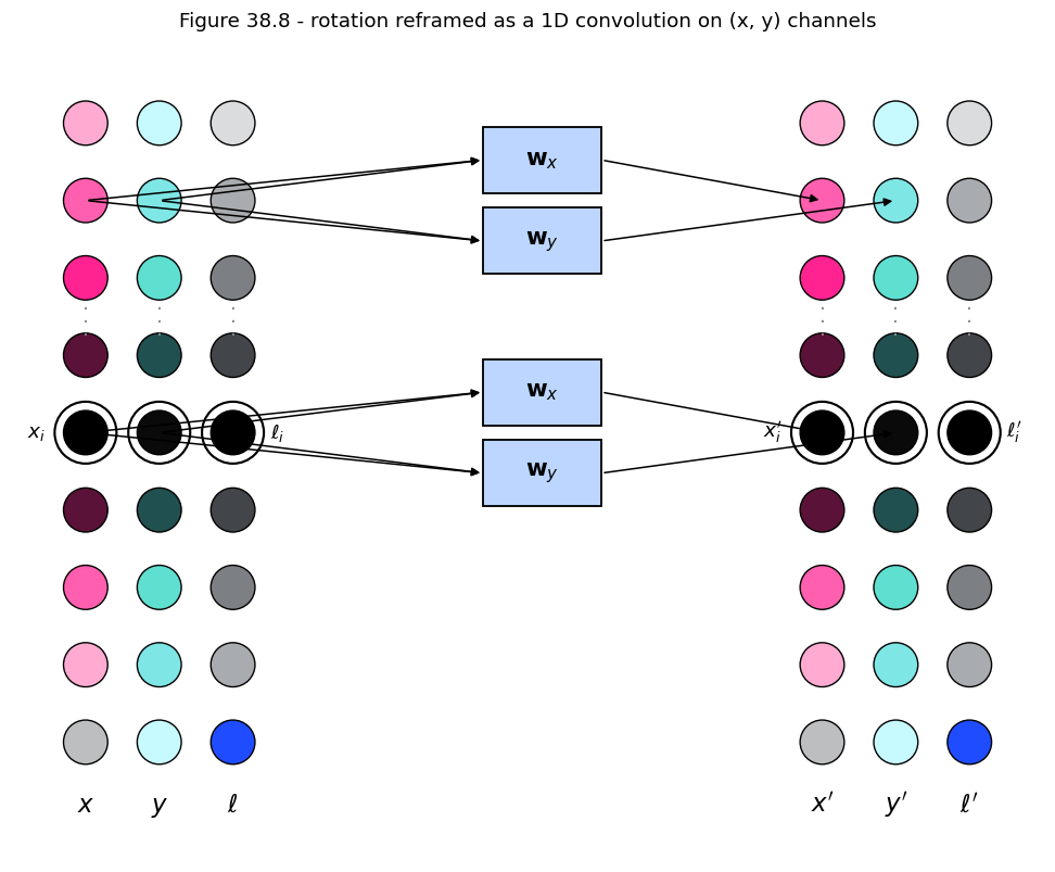
If you represent an image as a set of triples $\{(\ell_i, x_i, y_i)\}$ (intensity plus explicit position), then a rotation is a *1D convolution on the position channels*:
$\begin{bmatrix}x'\\y'\end{bmatrix} = \underbrace{\begin{bmatrix}\cos\theta & -\sin\theta\\\sin\theta & \cos\theta\end{bmatrix}}_{\text{kernels } w_x, w_y} \begin{bmatrix}x\\y\end{bmatrix}.$
Intensity passes through untouched; only the coordinate channels are mixed (figure 38.8). This framing makes it natural to learn warps with neural networks that operate on coordinate channels, and the rest of the section builds that bridge.
### Geometric transformation as a convolution
If you represent an image as a set of triples $\{(\ell_i, x_i, y_i)\}$ (intensity plus explicit position), then a rotation is a *1D convolution on the position channels*:
$\begin{bmatrix}x'\\y'\end{bmatrix} = \underbrace{\begin{bmatrix}\cos\theta & -\sin\theta\\\sin\theta & \cos\theta\end{bmatrix}}_{\text{kernels } w_x, w_y} \begin{bmatrix}x\\y\end{bmatrix}.$
Intensity passes through untouched; only the coordinate channels are mixed (figure 38.8). This framing makes it natural to learn warps with neural networks that operate on coordinate channels, and the rest of the section builds that bridge.
 ## Lines and points: cross-product duality
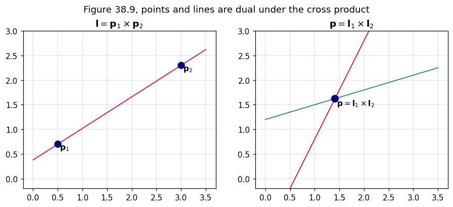
In homogeneous coordinates, a 2D line $ax + by + c = 0$ is the vector $\mathbf{l} = (a, b, c)$, and incidence is $\mathbf{l}^\top \mathbf{p} = 0$. Two operations turn out to be the **same** cross product:
$\mathbf{l} = \mathbf{p}_1 \times \mathbf{p}_2 \qquad \text{(line through two points)}$
$\mathbf{p} = \mathbf{l}_1 \times \mathbf{l}_2 \qquad \text{(intersection of two lines)}$
Parallel lines intersect at a point with $w = 0$: a *point at infinity*, the homogeneous form of a vanishing point. The section on [3D motion and its 2D projection](/aiml-common/lectures/3d-reconstruction/3d-motion-projection/index) uses exactly this construction.
## Lines and points: cross-product duality
In homogeneous coordinates, a 2D line $ax + by + c = 0$ is the vector $\mathbf{l} = (a, b, c)$, and incidence is $\mathbf{l}^\top \mathbf{p} = 0$. Two operations turn out to be the **same** cross product:
$\mathbf{l} = \mathbf{p}_1 \times \mathbf{p}_2 \qquad \text{(line through two points)}$
$\mathbf{p} = \mathbf{l}_1 \times \mathbf{l}_2 \qquad \text{(intersection of two lines)}$
Parallel lines intersect at a point with $w = 0$: a *point at infinity*, the homogeneous form of a vanishing point. The section on [3D motion and its 2D projection](/aiml-common/lectures/3d-reconstruction/3d-motion-projection/index) uses exactly this construction.
 ## Image warping: forward and backward mapping
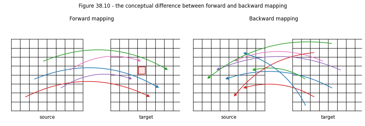
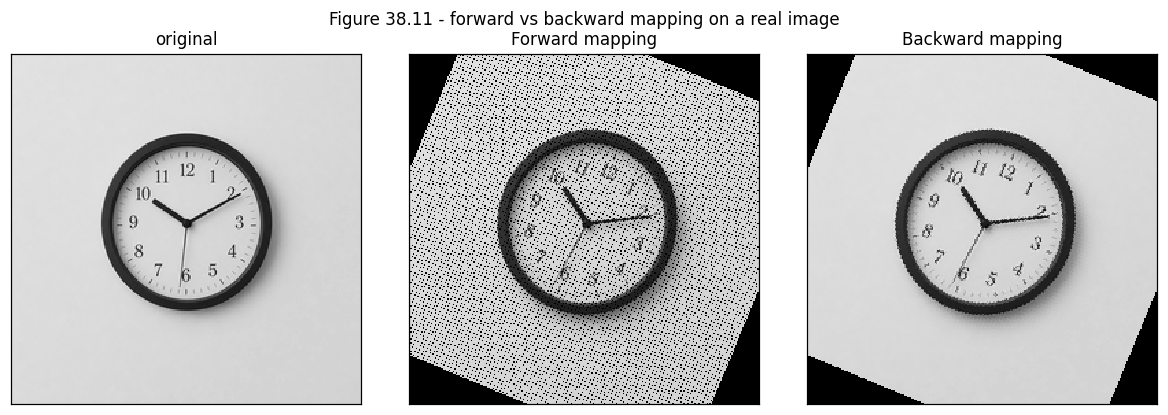
Applying a transformation $M$ to an image *should* give you a new image. The naive way, forward mapping, walks the input pixels, transforms each location, and writes its intensity to the nearest target pixel. That leaves **holes**, because an expansion spreads the input pixels too thinly to cover the target grid. The correct way, backward mapping, walks the *target* pixels and pulls each back through $M^{-1}$, so every output pixel gets one well-defined intensity (figures 38.10 and 38.11).
A small checkerboard makes the artifacts easy to see.
```python theme={null}
def make_checkerboard(n=80, squares=8):
"""Small checkerboard image as a tensor in [0, 1]."""
g = (torch.arange(n)[:, None] // (n // squares)) + (torch.arange(n)[None, :] // (n // squares))
return (g % 2).float()
def forward_warp(img, M):
"""Forward mapping with nearest-neighbor write. Produces holes."""
H, W = img.shape
out = torch.zeros_like(img)
ys, xs = torch.meshgrid(torch.arange(H), torch.arange(W), indexing="ij")
pts = torch.stack([xs.flatten().float(), ys.flatten().float()], dim=-1)
new = apply_T(M, pts).round().long()
new_x, new_y = new[:, 0], new[:, 1]
mask = (new_x >= 0) & (new_x < W) & (new_y >= 0) & (new_y < H)
out[new_y[mask], new_x[mask]] = img[ys.flatten()[mask], xs.flatten()[mask]]
return out
def backward_warp(img, M):
"""Backward mapping with nearest-neighbor sample. Hole-free."""
H, W = img.shape
Minv = torch.linalg.inv(M)
ys, xs = torch.meshgrid(torch.arange(H), torch.arange(W), indexing="ij")
pts = torch.stack([xs.flatten().float(), ys.flatten().float()], dim=-1)
src = apply_T(Minv, pts).round().long()
src_x, src_y = src[:, 0], src[:, 1]
mask = (src_x >= 0) & (src_x < W) & (src_y >= 0) & (src_y < H)
out = torch.zeros_like(img)
out.view(-1)[mask] = img[src_y[mask], src_x[mask]]
return out
```
## Image warping: forward and backward mapping
Applying a transformation $M$ to an image *should* give you a new image. The naive way, forward mapping, walks the input pixels, transforms each location, and writes its intensity to the nearest target pixel. That leaves **holes**, because an expansion spreads the input pixels too thinly to cover the target grid. The correct way, backward mapping, walks the *target* pixels and pulls each back through $M^{-1}$, so every output pixel gets one well-defined intensity (figures 38.10 and 38.11).
A small checkerboard makes the artifacts easy to see.
```python theme={null}
def make_checkerboard(n=80, squares=8):
"""Small checkerboard image as a tensor in [0, 1]."""
g = (torch.arange(n)[:, None] // (n // squares)) + (torch.arange(n)[None, :] // (n // squares))
return (g % 2).float()
def forward_warp(img, M):
"""Forward mapping with nearest-neighbor write. Produces holes."""
H, W = img.shape
out = torch.zeros_like(img)
ys, xs = torch.meshgrid(torch.arange(H), torch.arange(W), indexing="ij")
pts = torch.stack([xs.flatten().float(), ys.flatten().float()], dim=-1)
new = apply_T(M, pts).round().long()
new_x, new_y = new[:, 0], new[:, 1]
mask = (new_x >= 0) & (new_x < W) & (new_y >= 0) & (new_y < H)
out[new_y[mask], new_x[mask]] = img[ys.flatten()[mask], xs.flatten()[mask]]
return out
def backward_warp(img, M):
"""Backward mapping with nearest-neighbor sample. Hole-free."""
H, W = img.shape
Minv = torch.linalg.inv(M)
ys, xs = torch.meshgrid(torch.arange(H), torch.arange(W), indexing="ij")
pts = torch.stack([xs.flatten().float(), ys.flatten().float()], dim=-1)
src = apply_T(Minv, pts).round().long()
src_x, src_y = src[:, 0], src[:, 1]
mask = (src_x >= 0) & (src_x < W) & (src_y >= 0) & (src_y < H)
out = torch.zeros_like(img)
out.view(-1)[mask] = img[src_y[mask], src_x[mask]]
return out
```
 ### Differentiable warping with Kornia
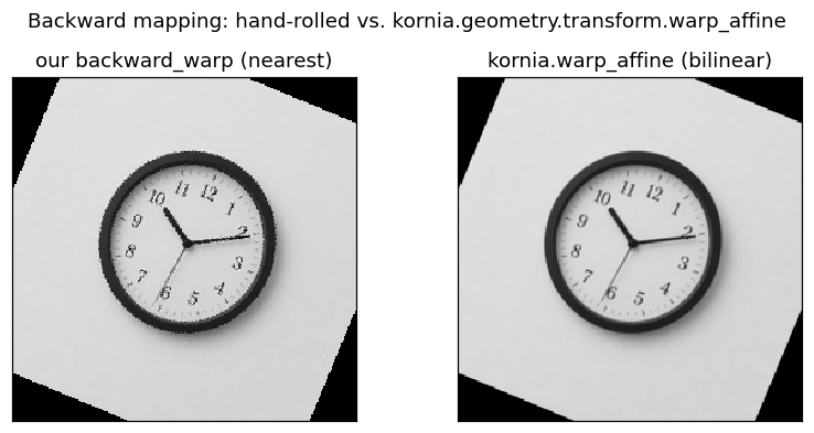
The hand-written `backward_warp` above shows the principle. In practice you use [Kornia](https://kornia.readthedocs.io/), a differentiable computer vision library built on PyTorch. Its `warp_affine` performs the same backward mapping, but with bilinear interpolation (so no nearest-neighbor aliasing), in batches, and differentiably end to end. The next cell feeds it the same matrix $M$ and compares the result with the hand-written version.
```python theme={null}
# kornia equivalent of backward_warp - bilinear, batched, differentiable.
# The clock image from above keeps the side-by-side on the same subject.
img_bchw = clock_img.unsqueeze(0).unsqueeze(0)
M_b23 = M[:2, :3].unsqueeze(0)
H, W = clock_img.shape
kornia_warp = KT.warp_affine(img_bchw, M_b23, dsize=(H, W), mode="bilinear")
kornia_warp = kornia_warp.squeeze(0).squeeze(0)
```
### Differentiable warping with Kornia
The hand-written `backward_warp` above shows the principle. In practice you use [Kornia](https://kornia.readthedocs.io/), a differentiable computer vision library built on PyTorch. Its `warp_affine` performs the same backward mapping, but with bilinear interpolation (so no nearest-neighbor aliasing), in batches, and differentiably end to end. The next cell feeds it the same matrix $M$ and compares the result with the hand-written version.
```python theme={null}
# kornia equivalent of backward_warp - bilinear, batched, differentiable.
# The clock image from above keeps the side-by-side on the same subject.
img_bchw = clock_img.unsqueeze(0).unsqueeze(0)
M_b23 = M[:2, :3].unsqueeze(0)
H, W = clock_img.shape
kornia_warp = KT.warp_affine(img_bchw, M_b23, dsize=(H, W), mode="bilinear")
kornia_warp = kornia_warp.squeeze(0).squeeze(0)
```
 ## Implicit image representations (SIREN)
Backward mapping at sub-pixel locations needs an interpolation kernel, but only because the image is stored as a discrete grid. **SIREN** (Sitzmann et al., NeurIPS 2020) does away with the grid: it represents an image as a small network $f_\theta : (x, y) \to \text{intensity}$ whose layers use $\sin$ activations. The trained network *is* the image, and you can evaluate it at any continuous coordinate.
Geometric warping then becomes a coordinate transform with no interpolation kernel:
$\hat\ell(x, y) = f_\theta(M^{-1}(x, y, 1)^\top).$
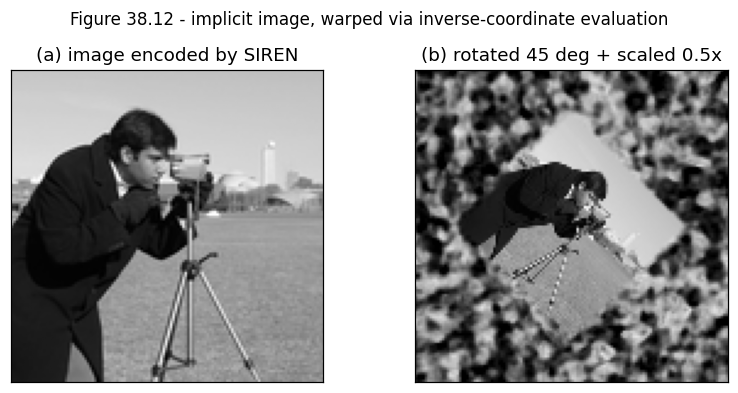
The next cells train a small SIREN on the cameraman test image and warp it by feeding pre-transformed coordinates (figure 38.12). The training is deliberately short: the point is to demonstrate the representation, not to maximize reconstruction quality.
```python theme={null}
class SIREN(nn.Module):
"""Tiny implicit image network. Sine-activated MLP per Sitzmann et al., 2020."""
def __init__(self, hidden=256, layers=4, w0=30.0):
super().__init__()
self.w0 = w0
net = [nn.Linear(2, hidden)]
for _ in range(layers - 1):
net.append(nn.Linear(hidden, hidden))
net.append(nn.Linear(hidden, 1))
self.net = nn.ModuleList(net)
self._init_weights()
def _init_weights(self):
with torch.no_grad():
self.net[0].weight.uniform_(-1 / 2, 1 / 2)
for layer in self.net[1:]:
bound = (6.0 / layer.in_features) ** 0.5 / self.w0
layer.weight.uniform_(-bound, bound)
def forward(self, xy):
h = torch.sin(self.w0 * self.net[0](xy))
for layer in self.net[1:-1]:
h = torch.sin(self.w0 * layer(h))
return self.net[-1](h)
def make_target_image(n=128):
"""Load the classic 'cameraman' test image (essentially what the book uses
for Figure 38.12), center-crop, and downsample to n x n in [0, 1]."""
cam = skimage.data.camera() # (512, 512) uint8
H, W = cam.shape
# Center-crop to square (already square, but stay explicit), then downsample
side = min(H, W)
cy0, cx0 = (H - side) // 2, (W - side) // 2
cropped = cam[cy0:cy0 + side, cx0:cx0 + side]
# Convert through PIL for nice resampling, then bytes -> torch (no numpy on the math side).
img = Image.fromarray(cropped, mode="L").resize((n, n), Image.LANCZOS)
pixels = torch.frombuffer(bytearray(img.tobytes()), dtype=torch.uint8)
return pixels.to(torch.float32).view(n, n) / 255.0
def coord_grid(n):
"""Regular [-1, 1]^2 grid of shape (n*n, 2)."""
ys = torch.linspace(-1, 1, n)
xs = torch.linspace(-1, 1, n)
yy, xx = torch.meshgrid(ys, xs, indexing="ij")
return torch.stack([xx.flatten(), yy.flatten()], dim=-1)
```
```python theme={null}
# Train SIREN on the cameraman image. Real images need more capacity / steps
# than a synthetic blob; 2000 steps with a slightly wider MLP gets a decent
# memorisation in ~10s on CPU.
N = 128
target = make_target_image(N).flatten().unsqueeze(-1)
grid = coord_grid(N)
model = SIREN(hidden=256, layers=4, w0=30.0)
optim = torch.optim.Adam(model.parameters(), lr=1e-4)
for step in range(2000):
pred = model(grid)
loss = ((pred - target) ** 2).mean()
optim.zero_grad()
loss.backward()
optim.step()
print(f"final reconstruction MSE: {loss.item():.4f}")
```
```output theme={null}
final reconstruction MSE: 0.0000
```
## Implicit image representations (SIREN)
Backward mapping at sub-pixel locations needs an interpolation kernel, but only because the image is stored as a discrete grid. **SIREN** (Sitzmann et al., NeurIPS 2020) does away with the grid: it represents an image as a small network $f_\theta : (x, y) \to \text{intensity}$ whose layers use $\sin$ activations. The trained network *is* the image, and you can evaluate it at any continuous coordinate.
Geometric warping then becomes a coordinate transform with no interpolation kernel:
$\hat\ell(x, y) = f_\theta(M^{-1}(x, y, 1)^\top).$
The next cells train a small SIREN on the cameraman test image and warp it by feeding pre-transformed coordinates (figure 38.12). The training is deliberately short: the point is to demonstrate the representation, not to maximize reconstruction quality.
```python theme={null}
class SIREN(nn.Module):
"""Tiny implicit image network. Sine-activated MLP per Sitzmann et al., 2020."""
def __init__(self, hidden=256, layers=4, w0=30.0):
super().__init__()
self.w0 = w0
net = [nn.Linear(2, hidden)]
for _ in range(layers - 1):
net.append(nn.Linear(hidden, hidden))
net.append(nn.Linear(hidden, 1))
self.net = nn.ModuleList(net)
self._init_weights()
def _init_weights(self):
with torch.no_grad():
self.net[0].weight.uniform_(-1 / 2, 1 / 2)
for layer in self.net[1:]:
bound = (6.0 / layer.in_features) ** 0.5 / self.w0
layer.weight.uniform_(-bound, bound)
def forward(self, xy):
h = torch.sin(self.w0 * self.net[0](xy))
for layer in self.net[1:-1]:
h = torch.sin(self.w0 * layer(h))
return self.net[-1](h)
def make_target_image(n=128):
"""Load the classic 'cameraman' test image (essentially what the book uses
for Figure 38.12), center-crop, and downsample to n x n in [0, 1]."""
cam = skimage.data.camera() # (512, 512) uint8
H, W = cam.shape
# Center-crop to square (already square, but stay explicit), then downsample
side = min(H, W)
cy0, cx0 = (H - side) // 2, (W - side) // 2
cropped = cam[cy0:cy0 + side, cx0:cx0 + side]
# Convert through PIL for nice resampling, then bytes -> torch (no numpy on the math side).
img = Image.fromarray(cropped, mode="L").resize((n, n), Image.LANCZOS)
pixels = torch.frombuffer(bytearray(img.tobytes()), dtype=torch.uint8)
return pixels.to(torch.float32).view(n, n) / 255.0
def coord_grid(n):
"""Regular [-1, 1]^2 grid of shape (n*n, 2)."""
ys = torch.linspace(-1, 1, n)
xs = torch.linspace(-1, 1, n)
yy, xx = torch.meshgrid(ys, xs, indexing="ij")
return torch.stack([xx.flatten(), yy.flatten()], dim=-1)
```
```python theme={null}
# Train SIREN on the cameraman image. Real images need more capacity / steps
# than a synthetic blob; 2000 steps with a slightly wider MLP gets a decent
# memorisation in ~10s on CPU.
N = 128
target = make_target_image(N).flatten().unsqueeze(-1)
grid = coord_grid(N)
model = SIREN(hidden=256, layers=4, w0=30.0)
optim = torch.optim.Adam(model.parameters(), lr=1e-4)
for step in range(2000):
pred = model(grid)
loss = ((pred - target) ** 2).mean()
optim.zero_grad()
loss.backward()
optim.step()
print(f"final reconstruction MSE: {loss.item():.4f}")
```
```output theme={null}
final reconstruction MSE: 0.0000
```
 ## Concluding remarks
The section moves forward one promotion at a time:
* **Heterogeneous to homogeneous**: every affine and projective transformation becomes a single matrix product.
* **Points and lines to cross-product duality**: incidence, joins, and intersections collapse into one operation. Parallel lines meet at points with $w=0$, so vanishing points get a coordinate.
* **Discrete grid to implicit function**: with SIREN, the image *is* its parameters. Warping becomes an inverse-coordinate query and interpolation kernels disappear.
Every later geometry chapter of the book (perspective projection in 39, stereo in 40, homographies in 41, single-view metrology in 42, structure from motion in 44, radiance fields in 45) reuses the homogeneous algebra and the point and line duality set up here.
***
[Edit this page on GitHub](https://github.com/aegean-ai/eaia/edit/main/src/aiml-common/lectures/3d-reconstruction/images-and-geometry/index.mdx) or [file an issue](https://github.com/aegean-ai/eaia/issues/new/choose).
## Concluding remarks
The section moves forward one promotion at a time:
* **Heterogeneous to homogeneous**: every affine and projective transformation becomes a single matrix product.
* **Points and lines to cross-product duality**: incidence, joins, and intersections collapse into one operation. Parallel lines meet at points with $w=0$, so vanishing points get a coordinate.
* **Discrete grid to implicit function**: with SIREN, the image *is* its parameters. Warping becomes an inverse-coordinate query and interpolation kernels disappear.
Every later geometry chapter of the book (perspective projection in 39, stereo in 40, homographies in 41, single-view metrology in 42, structure from motion in 44, radiance fields in 45) reuses the homogeneous algebra and the point and line duality set up here.
***
[Edit this page on GitHub](https://github.com/aegean-ai/eaia/edit/main/src/aiml-common/lectures/3d-reconstruction/images-and-geometry/index.mdx) or [file an issue](https://github.com/aegean-ai/eaia/issues/new/choose).