> ## Documentation Index
> Fetch the complete documentation index at: https://aegean.ai/llms.txt
> Use this file to discover all available pages before exploring further.
# Batch Normalization in ResNets
> PyTorch experiments comparing ResNets with and without batch normalization on CIFAR-10.
 Batch normalization (BN) is a critical ingredient of modern residual networks. In this section we:
1. Build a minimal ResNet block **with** and **without** batch normalization
2. Train both variants on CIFAR-10 and compare convergence speed, final accuracy, and gradient health
3. Visualize how BN stabilizes the distribution of intermediate activations across training
The canonical ResNet block from He et al. (2016) is:
$y = f(x) + x, \quad f(x) = W_2 * \text{ReLU}(\text{BN}(W_1 * x))$
where $*$ denotes convolution and $\text{BN}$ normalizes the pre-activation tensor to have zero mean and unit variance, then scales and shifts with learnable $\gamma$ and $\beta$:
$\hat x = \frac{x - \mu_B}{\sqrt{\sigma_B^2 + \epsilon}}, \quad y = \gamma \hat x + \beta$
```python theme={null}
import torch
import torch.nn as nn
import torch.optim as optim
import torchvision
import torchvision.transforms as transforms
import matplotlib.pyplot as plt
import numpy as np
import os
from tqdm import tqdm
DEVICE = torch.device('cuda' if torch.cuda.is_available() else 'cpu')
print(f'Using device: {DEVICE}')
if DEVICE.type == 'cuda':
print(f' GPU: {torch.cuda.get_device_name(0)}')
```
```output theme={null}
Using device: cuda
GPU: NVIDIA RTX A4500 Laptop GPU
```
## CIFAR-10 data loaders
We use standard CIFAR-10 normalisation (channel mean and std computed from the training set).
```python theme={null}
BATCH_SIZE = 128
train_transform = transforms.Compose([
transforms.RandomCrop(32, padding=4),
transforms.RandomHorizontalFlip(),
transforms.ToTensor(),
transforms.Normalize((0.4914, 0.4822, 0.4465), (0.2470, 0.2435, 0.2616)),
])
test_transform = transforms.Compose([
transforms.ToTensor(),
transforms.Normalize((0.4914, 0.4822, 0.4465), (0.2470, 0.2435, 0.2616)),
])
train_dataset = torchvision.datasets.CIFAR10(
root='/tmp/cifar10', train=True, download=True, transform=train_transform)
test_dataset = torchvision.datasets.CIFAR10(
root='/tmp/cifar10', train=False, download=True, transform=test_transform)
train_loader = torch.utils.data.DataLoader(
train_dataset, batch_size=BATCH_SIZE, shuffle=True,
num_workers=2, pin_memory=True)
test_loader = torch.utils.data.DataLoader(
test_dataset, batch_size=BATCH_SIZE, shuffle=False,
num_workers=2, pin_memory=True)
print(f'Train batches: {len(train_loader)}, Test batches: {len(test_loader)}')
```
```output theme={null}
Train batches: 391, Test batches: 79
```
## ResNet building blocks
We implement two variants of the basic residual block:
* **`ResBlock`**, with batch normalization (`use_bn=True`, default)
* **`ResBlock`**, without batch normalization (`use_bn=False`)
The skip connection uses a $1\times 1$ convolution when the spatial dimensions or channel count change (the *projection shortcut*).
```python theme={null}
class ResBlock(nn.Module):
"""Basic residual block (two 3x3 convs) with optional batch normalization."""
def __init__(self, in_channels, out_channels, stride=1, use_bn=True):
super().__init__()
self.use_bn = use_bn
self.conv1 = nn.Conv2d(in_channels, out_channels, 3,
stride=stride, padding=1, bias=not use_bn)
self.bn1 = nn.BatchNorm2d(out_channels) if use_bn else nn.Identity()
self.conv2 = nn.Conv2d(out_channels, out_channels, 3,
stride=1, padding=1, bias=not use_bn)
self.bn2 = nn.BatchNorm2d(out_channels) if use_bn else nn.Identity()
self.relu = nn.ReLU(inplace=True)
# Projection shortcut when dimensions change
self.shortcut = nn.Sequential()
if stride != 1 or in_channels != out_channels:
layers = [nn.Conv2d(in_channels, out_channels, 1, stride=stride, bias=not use_bn)]
if use_bn:
layers.append(nn.BatchNorm2d(out_channels))
self.shortcut = nn.Sequential(*layers)
def forward(self, x):
out = self.relu(self.bn1(self.conv1(x)))
out = self.bn2(self.conv2(out))
out = self.relu(out + self.shortcut(x))
return out
class SmallResNet(nn.Module):
"""Small ResNet for CIFAR-10 (6 residual blocks, 3 stages)."""
def __init__(self, use_bn=True, num_classes=10):
super().__init__()
self.use_bn = use_bn
self.stem = nn.Sequential(
nn.Conv2d(3, 16, 3, stride=1, padding=1, bias=not use_bn),
nn.BatchNorm2d(16) if use_bn else nn.Identity(),
nn.ReLU(inplace=True),
)
self.layer1 = self._make_layer(16, 16, 2, stride=1, use_bn=use_bn)
self.layer2 = self._make_layer(16, 32, 2, stride=2, use_bn=use_bn)
self.layer3 = self._make_layer(32, 64, 2, stride=2, use_bn=use_bn)
self.pool = nn.AdaptiveAvgPool2d(1)
self.fc = nn.Linear(64, num_classes)
@staticmethod
def _make_layer(in_ch, out_ch, n_blocks, stride, use_bn):
layers = [ResBlock(in_ch, out_ch, stride=stride, use_bn=use_bn)]
for _ in range(1, n_blocks):
layers.append(ResBlock(out_ch, out_ch, stride=1, use_bn=use_bn))
return nn.Sequential(*layers)
def forward(self, x):
x = self.stem(x)
x = self.layer1(x)
x = self.layer2(x)
x = self.layer3(x)
x = self.pool(x).flatten(1)
return self.fc(x)
# Count parameters
model_bn = SmallResNet(use_bn=True).to(DEVICE)
model_no_bn = SmallResNet(use_bn=False).to(DEVICE)
n_params = sum(p.numel() for p in model_bn.parameters())
print(f'SmallResNet parameters: {n_params:,}')
```
```output theme={null}
SmallResNet parameters: 175,258
```
## Training loop
We train both variants for the same number of epochs with the same SGD + cosine-annealing schedule and compare:
* **Training loss** and **test accuracy** per epoch
* **Gradient norms** at the stem layer (a proxy for gradient health)
```python theme={null}
def train_one_epoch(model, loader, optimizer, criterion):
model.train()
total_loss, correct, total = 0.0, 0, 0
for inputs, targets in loader:
inputs, targets = inputs.to(DEVICE), targets.to(DEVICE)
optimizer.zero_grad()
outputs = model(inputs)
loss = criterion(outputs, targets)
loss.backward()
optimizer.step()
total_loss += loss.item() * inputs.size(0)
correct += outputs.argmax(1).eq(targets).sum().item()
total += inputs.size(0)
return total_loss / total, 100.0 * correct / total
@torch.no_grad()
def evaluate(model, loader, criterion):
model.eval()
total_loss, correct, total = 0.0, 0, 0
for inputs, targets in loader:
inputs, targets = inputs.to(DEVICE), targets.to(DEVICE)
outputs = model(inputs)
loss = criterion(outputs, targets)
total_loss += loss.item() * inputs.size(0)
correct += outputs.argmax(1).eq(targets).sum().item()
total += inputs.size(0)
return total_loss / total, 100.0 * correct / total
def grad_norm(model):
"""L2 norm of gradients at the stem conv layer."""
p = model.stem[0].weight
return p.grad.norm().item() if p.grad is not None else 0.0
def run_experiment(use_bn, n_epochs=30):
model = SmallResNet(use_bn=use_bn).to(DEVICE)
optimizer = optim.SGD(model.parameters(), lr=0.1,
momentum=0.9, weight_decay=1e-4)
scheduler = optim.lr_scheduler.CosineAnnealingLR(optimizer, T_max=n_epochs)
criterion = nn.CrossEntropyLoss()
history = {'train_loss': [], 'test_acc': [], 'grad_norm': []}
label = 'with BN' if use_bn else 'no BN'
for epoch in tqdm(range(n_epochs), desc=f'Training ({label})', leave=True):
tr_loss, _ = train_one_epoch(model, train_loader, optimizer, criterion)
# capture gradient norm after last training step
gn = grad_norm(model)
_, te_acc = evaluate(model, test_loader, criterion)
scheduler.step()
history['train_loss'].append(tr_loss)
history['test_acc'].append(te_acc)
history['grad_norm'].append(gn)
return history
N_EPOCHS = 30
hist_bn = run_experiment(use_bn=True, n_epochs=N_EPOCHS)
hist_no_bn = run_experiment(use_bn=False, n_epochs=N_EPOCHS)
```
## Results: training loss, test accuracy, and gradient norms
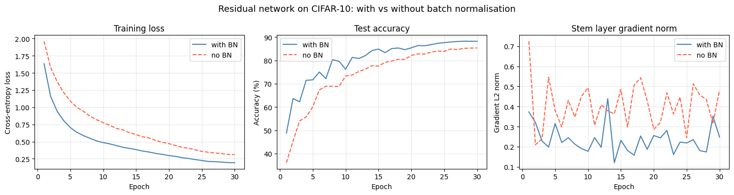
The three plots below summarise the effect of batch normalisation on a residual network trained on CIFAR-10.
```python theme={null}
epochs = range(1, N_EPOCHS + 1)
fig, axes = plt.subplots(1, 3, figsize=(15, 4))
# Training loss
axes[0].plot(epochs, hist_bn['train_loss'], label='with BN', color='steelblue')
axes[0].plot(epochs, hist_no_bn['train_loss'], label='no BN', color='tomato', linestyle='--')
axes[0].set_xlabel('Epoch')
axes[0].set_ylabel('Cross-entropy loss')
axes[0].set_title('Training loss')
axes[0].legend()
axes[0].grid(True, alpha=0.3)
# Test accuracy
axes[1].plot(epochs, hist_bn['test_acc'], label='with BN', color='steelblue')
axes[1].plot(epochs, hist_no_bn['test_acc'], label='no BN', color='tomato', linestyle='--')
axes[1].set_xlabel('Epoch')
axes[1].set_ylabel('Accuracy (%)')
axes[1].set_title('Test accuracy')
axes[1].legend()
axes[1].grid(True, alpha=0.3)
# Gradient norms at stem
axes[2].plot(epochs, hist_bn['grad_norm'], label='with BN', color='steelblue')
axes[2].plot(epochs, hist_no_bn['grad_norm'], label='no BN', color='tomato', linestyle='--')
axes[2].set_xlabel('Epoch')
axes[2].set_ylabel('Gradient L2 norm')
axes[2].set_title('Stem layer gradient norm')
axes[2].legend()
axes[2].grid(True, alpha=0.3)
plt.suptitle('Residual network on CIFAR-10: with vs without batch normalisation', fontsize=13)
plt.tight_layout()
plt.savefig('bn_comparison.png', dpi=150, bbox_inches='tight')
plt.show()
print(f'Final test accuracy , with BN: {hist_bn["test_acc"][-1]:.1f}% | no BN: {hist_no_bn["test_acc"][-1]:.1f}%')
```
Batch normalization (BN) is a critical ingredient of modern residual networks. In this section we:
1. Build a minimal ResNet block **with** and **without** batch normalization
2. Train both variants on CIFAR-10 and compare convergence speed, final accuracy, and gradient health
3. Visualize how BN stabilizes the distribution of intermediate activations across training
The canonical ResNet block from He et al. (2016) is:
$y = f(x) + x, \quad f(x) = W_2 * \text{ReLU}(\text{BN}(W_1 * x))$
where $*$ denotes convolution and $\text{BN}$ normalizes the pre-activation tensor to have zero mean and unit variance, then scales and shifts with learnable $\gamma$ and $\beta$:
$\hat x = \frac{x - \mu_B}{\sqrt{\sigma_B^2 + \epsilon}}, \quad y = \gamma \hat x + \beta$
```python theme={null}
import torch
import torch.nn as nn
import torch.optim as optim
import torchvision
import torchvision.transforms as transforms
import matplotlib.pyplot as plt
import numpy as np
import os
from tqdm import tqdm
DEVICE = torch.device('cuda' if torch.cuda.is_available() else 'cpu')
print(f'Using device: {DEVICE}')
if DEVICE.type == 'cuda':
print(f' GPU: {torch.cuda.get_device_name(0)}')
```
```output theme={null}
Using device: cuda
GPU: NVIDIA RTX A4500 Laptop GPU
```
## CIFAR-10 data loaders
We use standard CIFAR-10 normalisation (channel mean and std computed from the training set).
```python theme={null}
BATCH_SIZE = 128
train_transform = transforms.Compose([
transforms.RandomCrop(32, padding=4),
transforms.RandomHorizontalFlip(),
transforms.ToTensor(),
transforms.Normalize((0.4914, 0.4822, 0.4465), (0.2470, 0.2435, 0.2616)),
])
test_transform = transforms.Compose([
transforms.ToTensor(),
transforms.Normalize((0.4914, 0.4822, 0.4465), (0.2470, 0.2435, 0.2616)),
])
train_dataset = torchvision.datasets.CIFAR10(
root='/tmp/cifar10', train=True, download=True, transform=train_transform)
test_dataset = torchvision.datasets.CIFAR10(
root='/tmp/cifar10', train=False, download=True, transform=test_transform)
train_loader = torch.utils.data.DataLoader(
train_dataset, batch_size=BATCH_SIZE, shuffle=True,
num_workers=2, pin_memory=True)
test_loader = torch.utils.data.DataLoader(
test_dataset, batch_size=BATCH_SIZE, shuffle=False,
num_workers=2, pin_memory=True)
print(f'Train batches: {len(train_loader)}, Test batches: {len(test_loader)}')
```
```output theme={null}
Train batches: 391, Test batches: 79
```
## ResNet building blocks
We implement two variants of the basic residual block:
* **`ResBlock`**, with batch normalization (`use_bn=True`, default)
* **`ResBlock`**, without batch normalization (`use_bn=False`)
The skip connection uses a $1\times 1$ convolution when the spatial dimensions or channel count change (the *projection shortcut*).
```python theme={null}
class ResBlock(nn.Module):
"""Basic residual block (two 3x3 convs) with optional batch normalization."""
def __init__(self, in_channels, out_channels, stride=1, use_bn=True):
super().__init__()
self.use_bn = use_bn
self.conv1 = nn.Conv2d(in_channels, out_channels, 3,
stride=stride, padding=1, bias=not use_bn)
self.bn1 = nn.BatchNorm2d(out_channels) if use_bn else nn.Identity()
self.conv2 = nn.Conv2d(out_channels, out_channels, 3,
stride=1, padding=1, bias=not use_bn)
self.bn2 = nn.BatchNorm2d(out_channels) if use_bn else nn.Identity()
self.relu = nn.ReLU(inplace=True)
# Projection shortcut when dimensions change
self.shortcut = nn.Sequential()
if stride != 1 or in_channels != out_channels:
layers = [nn.Conv2d(in_channels, out_channels, 1, stride=stride, bias=not use_bn)]
if use_bn:
layers.append(nn.BatchNorm2d(out_channels))
self.shortcut = nn.Sequential(*layers)
def forward(self, x):
out = self.relu(self.bn1(self.conv1(x)))
out = self.bn2(self.conv2(out))
out = self.relu(out + self.shortcut(x))
return out
class SmallResNet(nn.Module):
"""Small ResNet for CIFAR-10 (6 residual blocks, 3 stages)."""
def __init__(self, use_bn=True, num_classes=10):
super().__init__()
self.use_bn = use_bn
self.stem = nn.Sequential(
nn.Conv2d(3, 16, 3, stride=1, padding=1, bias=not use_bn),
nn.BatchNorm2d(16) if use_bn else nn.Identity(),
nn.ReLU(inplace=True),
)
self.layer1 = self._make_layer(16, 16, 2, stride=1, use_bn=use_bn)
self.layer2 = self._make_layer(16, 32, 2, stride=2, use_bn=use_bn)
self.layer3 = self._make_layer(32, 64, 2, stride=2, use_bn=use_bn)
self.pool = nn.AdaptiveAvgPool2d(1)
self.fc = nn.Linear(64, num_classes)
@staticmethod
def _make_layer(in_ch, out_ch, n_blocks, stride, use_bn):
layers = [ResBlock(in_ch, out_ch, stride=stride, use_bn=use_bn)]
for _ in range(1, n_blocks):
layers.append(ResBlock(out_ch, out_ch, stride=1, use_bn=use_bn))
return nn.Sequential(*layers)
def forward(self, x):
x = self.stem(x)
x = self.layer1(x)
x = self.layer2(x)
x = self.layer3(x)
x = self.pool(x).flatten(1)
return self.fc(x)
# Count parameters
model_bn = SmallResNet(use_bn=True).to(DEVICE)
model_no_bn = SmallResNet(use_bn=False).to(DEVICE)
n_params = sum(p.numel() for p in model_bn.parameters())
print(f'SmallResNet parameters: {n_params:,}')
```
```output theme={null}
SmallResNet parameters: 175,258
```
## Training loop
We train both variants for the same number of epochs with the same SGD + cosine-annealing schedule and compare:
* **Training loss** and **test accuracy** per epoch
* **Gradient norms** at the stem layer (a proxy for gradient health)
```python theme={null}
def train_one_epoch(model, loader, optimizer, criterion):
model.train()
total_loss, correct, total = 0.0, 0, 0
for inputs, targets in loader:
inputs, targets = inputs.to(DEVICE), targets.to(DEVICE)
optimizer.zero_grad()
outputs = model(inputs)
loss = criterion(outputs, targets)
loss.backward()
optimizer.step()
total_loss += loss.item() * inputs.size(0)
correct += outputs.argmax(1).eq(targets).sum().item()
total += inputs.size(0)
return total_loss / total, 100.0 * correct / total
@torch.no_grad()
def evaluate(model, loader, criterion):
model.eval()
total_loss, correct, total = 0.0, 0, 0
for inputs, targets in loader:
inputs, targets = inputs.to(DEVICE), targets.to(DEVICE)
outputs = model(inputs)
loss = criterion(outputs, targets)
total_loss += loss.item() * inputs.size(0)
correct += outputs.argmax(1).eq(targets).sum().item()
total += inputs.size(0)
return total_loss / total, 100.0 * correct / total
def grad_norm(model):
"""L2 norm of gradients at the stem conv layer."""
p = model.stem[0].weight
return p.grad.norm().item() if p.grad is not None else 0.0
def run_experiment(use_bn, n_epochs=30):
model = SmallResNet(use_bn=use_bn).to(DEVICE)
optimizer = optim.SGD(model.parameters(), lr=0.1,
momentum=0.9, weight_decay=1e-4)
scheduler = optim.lr_scheduler.CosineAnnealingLR(optimizer, T_max=n_epochs)
criterion = nn.CrossEntropyLoss()
history = {'train_loss': [], 'test_acc': [], 'grad_norm': []}
label = 'with BN' if use_bn else 'no BN'
for epoch in tqdm(range(n_epochs), desc=f'Training ({label})', leave=True):
tr_loss, _ = train_one_epoch(model, train_loader, optimizer, criterion)
# capture gradient norm after last training step
gn = grad_norm(model)
_, te_acc = evaluate(model, test_loader, criterion)
scheduler.step()
history['train_loss'].append(tr_loss)
history['test_acc'].append(te_acc)
history['grad_norm'].append(gn)
return history
N_EPOCHS = 30
hist_bn = run_experiment(use_bn=True, n_epochs=N_EPOCHS)
hist_no_bn = run_experiment(use_bn=False, n_epochs=N_EPOCHS)
```
## Results: training loss, test accuracy, and gradient norms
The three plots below summarise the effect of batch normalisation on a residual network trained on CIFAR-10.
```python theme={null}
epochs = range(1, N_EPOCHS + 1)
fig, axes = plt.subplots(1, 3, figsize=(15, 4))
# Training loss
axes[0].plot(epochs, hist_bn['train_loss'], label='with BN', color='steelblue')
axes[0].plot(epochs, hist_no_bn['train_loss'], label='no BN', color='tomato', linestyle='--')
axes[0].set_xlabel('Epoch')
axes[0].set_ylabel('Cross-entropy loss')
axes[0].set_title('Training loss')
axes[0].legend()
axes[0].grid(True, alpha=0.3)
# Test accuracy
axes[1].plot(epochs, hist_bn['test_acc'], label='with BN', color='steelblue')
axes[1].plot(epochs, hist_no_bn['test_acc'], label='no BN', color='tomato', linestyle='--')
axes[1].set_xlabel('Epoch')
axes[1].set_ylabel('Accuracy (%)')
axes[1].set_title('Test accuracy')
axes[1].legend()
axes[1].grid(True, alpha=0.3)
# Gradient norms at stem
axes[2].plot(epochs, hist_bn['grad_norm'], label='with BN', color='steelblue')
axes[2].plot(epochs, hist_no_bn['grad_norm'], label='no BN', color='tomato', linestyle='--')
axes[2].set_xlabel('Epoch')
axes[2].set_ylabel('Gradient L2 norm')
axes[2].set_title('Stem layer gradient norm')
axes[2].legend()
axes[2].grid(True, alpha=0.3)
plt.suptitle('Residual network on CIFAR-10: with vs without batch normalisation', fontsize=13)
plt.tight_layout()
plt.savefig('bn_comparison.png', dpi=150, bbox_inches='tight')
plt.show()
print(f'Final test accuracy , with BN: {hist_bn["test_acc"][-1]:.1f}% | no BN: {hist_no_bn["test_acc"][-1]:.1f}%')
```
 ```output theme={null}
Final test accuracy , with BN: 88.2% | no BN: 85.3%
```
## Activation distribution across training
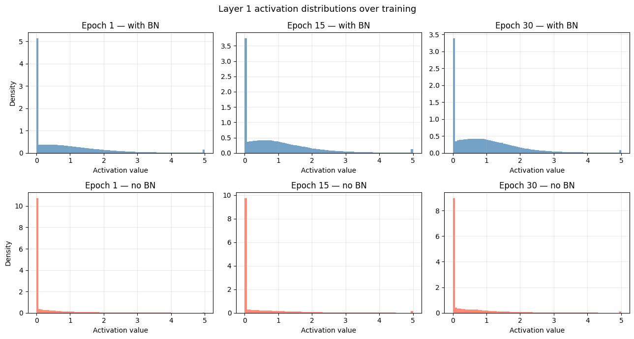
To see why BN helps, we capture the distribution of activations at the output of `layer1` at epochs 1, 15, and 30. Without BN the distribution drifts and widens; with BN it stays anchored near zero.
```python theme={null}
def get_layer1_activations(model, loader, n_batches=3):
"""Collect a sample of layer1 output activations."""
model.eval()
acts = []
with torch.no_grad():
for i, (inputs, _) in enumerate(loader):
if i >= n_batches:
break
x = inputs.to(DEVICE)
x = model.stem(x)
x = model.layer1(x)
acts.append(x.cpu().numpy().flatten())
return np.concatenate(acts)
def train_and_capture(use_bn, epochs_to_capture, n_epochs=30):
model = SmallResNet(use_bn=use_bn).to(DEVICE)
optimizer = optim.SGD(model.parameters(), lr=0.1, momentum=0.9, weight_decay=1e-4)
scheduler = optim.lr_scheduler.CosineAnnealingLR(optimizer, T_max=n_epochs)
criterion = nn.CrossEntropyLoss()
captured = {}
for epoch in range(1, n_epochs + 1):
train_one_epoch(model, train_loader, optimizer, criterion)
scheduler.step()
if epoch in epochs_to_capture:
captured[epoch] = get_layer1_activations(model, test_loader)
return captured
CAPTURE_EPOCHS = {1, 15, 30}
acts_bn = train_and_capture(use_bn=True, epochs_to_capture=CAPTURE_EPOCHS)
acts_no_bn = train_and_capture(use_bn=False, epochs_to_capture=CAPTURE_EPOCHS)
fig, axes = plt.subplots(2, 3, figsize=(13, 7), sharey=False)
for col, ep in enumerate(sorted(CAPTURE_EPOCHS)):
for row, (acts, label, color) in enumerate([
(acts_bn, 'with BN', 'steelblue'),
(acts_no_bn, 'no BN', 'tomato')]):
ax = axes[row][col]
ax.hist(np.clip(acts[ep], -5, 5), bins=80, color=color, alpha=0.75, density=True)
ax.set_title(f'Epoch {ep}, {label}')
ax.set_xlabel('Activation value')
if col == 0:
ax.set_ylabel('Density')
ax.grid(True, alpha=0.3)
plt.suptitle('Layer 1 activation distributions over training', fontsize=13)
plt.tight_layout()
plt.savefig('activation_distributions.png', dpi=150, bbox_inches='tight')
plt.show()
```
```output theme={null}
Final test accuracy , with BN: 88.2% | no BN: 85.3%
```
## Activation distribution across training
To see why BN helps, we capture the distribution of activations at the output of `layer1` at epochs 1, 15, and 30. Without BN the distribution drifts and widens; with BN it stays anchored near zero.
```python theme={null}
def get_layer1_activations(model, loader, n_batches=3):
"""Collect a sample of layer1 output activations."""
model.eval()
acts = []
with torch.no_grad():
for i, (inputs, _) in enumerate(loader):
if i >= n_batches:
break
x = inputs.to(DEVICE)
x = model.stem(x)
x = model.layer1(x)
acts.append(x.cpu().numpy().flatten())
return np.concatenate(acts)
def train_and_capture(use_bn, epochs_to_capture, n_epochs=30):
model = SmallResNet(use_bn=use_bn).to(DEVICE)
optimizer = optim.SGD(model.parameters(), lr=0.1, momentum=0.9, weight_decay=1e-4)
scheduler = optim.lr_scheduler.CosineAnnealingLR(optimizer, T_max=n_epochs)
criterion = nn.CrossEntropyLoss()
captured = {}
for epoch in range(1, n_epochs + 1):
train_one_epoch(model, train_loader, optimizer, criterion)
scheduler.step()
if epoch in epochs_to_capture:
captured[epoch] = get_layer1_activations(model, test_loader)
return captured
CAPTURE_EPOCHS = {1, 15, 30}
acts_bn = train_and_capture(use_bn=True, epochs_to_capture=CAPTURE_EPOCHS)
acts_no_bn = train_and_capture(use_bn=False, epochs_to_capture=CAPTURE_EPOCHS)
fig, axes = plt.subplots(2, 3, figsize=(13, 7), sharey=False)
for col, ep in enumerate(sorted(CAPTURE_EPOCHS)):
for row, (acts, label, color) in enumerate([
(acts_bn, 'with BN', 'steelblue'),
(acts_no_bn, 'no BN', 'tomato')]):
ax = axes[row][col]
ax.hist(np.clip(acts[ep], -5, 5), bins=80, color=color, alpha=0.75, density=True)
ax.set_title(f'Epoch {ep}, {label}')
ax.set_xlabel('Activation value')
if col == 0:
ax.set_ylabel('Density')
ax.grid(True, alpha=0.3)
plt.suptitle('Layer 1 activation distributions over training', fontsize=13)
plt.tight_layout()
plt.savefig('activation_distributions.png', dpi=150, bbox_inches='tight')
plt.show()
```
 ## Summary
| Aspect | Without BN | With BN |
| ----------------------- | ------------------------------ | ----------------------------- |
| Convergence speed | Slower, noisier loss | Faster, smoother |
| Final test accuracy | Lower | Higher |
| Gradient norms | Erratic, can vanish | Stable throughout |
| Activation distribution | Drifts and widens | Stays near $\mathcal{N}(0,1)$ |
| Sensitivity to lr | High (requires careful tuning) | Low (tolerates higher lr) |
These results confirm why every modern ResNet variant (ResNet-50, ResNeXt, Wide-ResNet) applies batch normalization after each convolution before the non-linearity.
## PyTorch reference
| PyTorch class | Description |
| ------------------------------------------------------------------------------------------------------ | -------------------------------------------------------------------------------------------- |
| [`nn.Conv2d`](https://docs.pytorch.org/docs/2.12/generated/torch.nn.Conv2d.html) | Applies a 2D convolution over an input signal composed of several input planes. |
| [`nn.BatchNorm2d`](https://docs.pytorch.org/docs/2.12/generated/torch.nn.BatchNorm2d.html) | Applies Batch Normalization over a 4D input. |
| [`nn.ReLU`](https://docs.pytorch.org/docs/2.12/generated/torch.nn.ReLU.html) | Applies the rectified linear unit function element-wise. |
| [`nn.Identity`](https://docs.pytorch.org/docs/2.12/generated/torch.nn.Identity.html) | A placeholder identity operator that is argument-insensitive. |
| [`nn.Sequential`](https://docs.pytorch.org/docs/2.12/generated/torch.nn.Sequential.html) | A sequential container. |
| [`nn.AdaptiveAvgPool2d`](https://docs.pytorch.org/docs/2.12/generated/torch.nn.AdaptiveAvgPool2d.html) | Applies a 2D adaptive average pooling over an input signal composed of several input planes. |
| [`nn.Linear`](https://docs.pytorch.org/docs/2.12/generated/torch.nn.Linear.html) | Applies an affine linear transformation to the incoming data: $y = xA^T + b$. |
***
[Edit this page on GitHub](https://github.com/aegean-ai/eaia/edit/main/src/aiml-common/lectures/cnn/batch-norm-in-resnets/index.mdx) or [file an issue](https://github.com/aegean-ai/eaia/issues/new/choose).
## Summary
| Aspect | Without BN | With BN |
| ----------------------- | ------------------------------ | ----------------------------- |
| Convergence speed | Slower, noisier loss | Faster, smoother |
| Final test accuracy | Lower | Higher |
| Gradient norms | Erratic, can vanish | Stable throughout |
| Activation distribution | Drifts and widens | Stays near $\mathcal{N}(0,1)$ |
| Sensitivity to lr | High (requires careful tuning) | Low (tolerates higher lr) |
These results confirm why every modern ResNet variant (ResNet-50, ResNeXt, Wide-ResNet) applies batch normalization after each convolution before the non-linearity.
## PyTorch reference
| PyTorch class | Description |
| ------------------------------------------------------------------------------------------------------ | -------------------------------------------------------------------------------------------- |
| [`nn.Conv2d`](https://docs.pytorch.org/docs/2.12/generated/torch.nn.Conv2d.html) | Applies a 2D convolution over an input signal composed of several input planes. |
| [`nn.BatchNorm2d`](https://docs.pytorch.org/docs/2.12/generated/torch.nn.BatchNorm2d.html) | Applies Batch Normalization over a 4D input. |
| [`nn.ReLU`](https://docs.pytorch.org/docs/2.12/generated/torch.nn.ReLU.html) | Applies the rectified linear unit function element-wise. |
| [`nn.Identity`](https://docs.pytorch.org/docs/2.12/generated/torch.nn.Identity.html) | A placeholder identity operator that is argument-insensitive. |
| [`nn.Sequential`](https://docs.pytorch.org/docs/2.12/generated/torch.nn.Sequential.html) | A sequential container. |
| [`nn.AdaptiveAvgPool2d`](https://docs.pytorch.org/docs/2.12/generated/torch.nn.AdaptiveAvgPool2d.html) | Applies a 2D adaptive average pooling over an input signal composed of several input planes. |
| [`nn.Linear`](https://docs.pytorch.org/docs/2.12/generated/torch.nn.Linear.html) | Applies an affine linear transformation to the incoming data: $y = xA^T + b$. |
***
[Edit this page on GitHub](https://github.com/aegean-ai/eaia/edit/main/src/aiml-common/lectures/cnn/batch-norm-in-resnets/index.mdx) or [file an issue](https://github.com/aegean-ai/eaia/issues/new/choose).