> ## Documentation Index
> Fetch the complete documentation index at: https://aegean.ai/llms.txt
> Use this file to discover all available pages before exploring further.
# Brownian motion, the continuous-time core of diffusion
> Visualize Brownian motion and connect it to the forward process of DDPM/DDIM.
Every diffusion model (DDPM, DDIM, score SDEs) has Brownian motion at its core. The discrete forward chain you saw in the [DDPM tutorial](/aiml-common/lectures/diffusion/ddpm/ddpm_mog_tutorial), clusters dissolving into Gaussian noise, is the discretization of a **continuous-time Wiener process**. Building intuition for the Wiener process makes the rest of the diffusion-model machinery click.
## Math recap: the Wiener process
A standard Wiener process $W_t$ on $[0, T]$ is a continuous-time stochastic process satisfying:
* $W_0 = 0$
* Independent increments: for $0 \le s < t$, $W_t - W_s \sim \mathcal{N}(0, t - s)$, independent of the path up to time $s$
* Continuous paths
A discrete-time approximation with step $\Delta t$ is the **random walk**
$W_{t + \Delta t} = W_t + \sqrt{\Delta t}\; \xi, \quad \xi \sim \mathcal{N}(0, 1)$
Multiplied by a diffusion coefficient $\sigma$ this gives Brownian motion with variance $\sigma^2 t$.
The DDPM forward chain $q(x_t \mid x_{t-1}) = \mathcal{N}(x_t; \sqrt{1-\beta_t}\, x_{t-1}, \beta_t I)$ is a *variance-preserving* discrete-time analogue: it adds Brownian-style noise *and* shrinks the signal each step so the marginal stays bounded.
## Brownian motion in motion
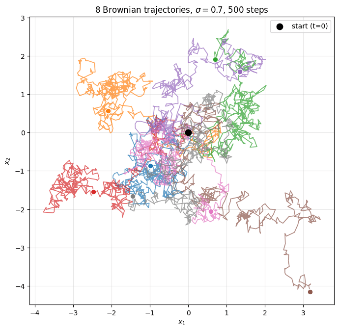
Eight particles released from the origin, each tracing an independent random walk. The trail behind each particle is its history, short trajectories on either side of the origin diverge into the wider variance the longer the chain runs.
## Eight Brownian trajectories
Eight particles released from the origin, each undergoing an independent random walk over 500 steps with $\sigma = 0.7$ and $\Delta t = 1/60$. The colored end-dots mark each trajectory's final position; the black dot at the origin marks the common start.
```python theme={null}
import numpy as np
import matplotlib.pyplot as plt
rng = np.random.default_rng(42)
n_particles = 8
n_steps = 500
dt = 1.0 / 60
sigma = 0.7
increments = sigma * np.sqrt(dt) * rng.standard_normal((n_steps + 1, n_particles, 2))
increments[0] = 0.0
paths = np.cumsum(increments, axis=0)
```
 ## Snapshot grid at the same timesteps as the DDPM forward process
200 fresh particles released from the origin, snapshotted at $t = 0, 10, 50, 100, 200, 500$, the same timesteps the [DDPM tutorial](/aiml-common/lectures/diffusion/ddpm/ddpm_mog_tutorial) uses for its forward-noising visualization. The cloud spreads with variance proportional to $t$, the hallmark of a Wiener process.
```python theme={null}
rng = np.random.default_rng(0)
n = 200
T = 500
snapshots = [0, 10, 50, 100, 200, 500]
sigma_grid = 0.5
increments = sigma_grid * np.sqrt(dt) * rng.standard_normal((T + 1, n, 2))
increments[0] = 0.0
grid_paths = np.cumsum(increments, axis=0)
```
## Snapshot grid at the same timesteps as the DDPM forward process
200 fresh particles released from the origin, snapshotted at $t = 0, 10, 50, 100, 200, 500$, the same timesteps the [DDPM tutorial](/aiml-common/lectures/diffusion/ddpm/ddpm_mog_tutorial) uses for its forward-noising visualization. The cloud spreads with variance proportional to $t$, the hallmark of a Wiener process.
```python theme={null}
rng = np.random.default_rng(0)
n = 200
T = 500
snapshots = [0, 10, 50, 100, 200, 500]
sigma_grid = 0.5
increments = sigma_grid * np.sqrt(dt) * rng.standard_normal((T + 1, n, 2))
increments[0] = 0.0
grid_paths = np.cumsum(increments, axis=0)
```
 ## Connection back to diffusion
Continuous-time diffusion frames the forward process as the SDE
$dx_t = f(x_t, t)\, dt + g(t)\, dW_t$
where $W_t$ is exactly the Brownian motion above. The **variance-preserving** SDE used by DDPM picks $f(x_t, t) = -\tfrac{1}{2}\beta(t)\, x_t$ and $g(t) = \sqrt{\beta(t)}$, so the marginal stays Gaussian and the variance is bounded. The discrete chain you trained earlier is the Euler-Maruyama discretization of this SDE.
Two takeaways:
* **Forward = Brownian motion + drift.** Everything diffusion-model-related sits on this foundation.
* **Reverse = score-based ODE/SDE.** Anderson's reverse-time SDE is what your trained $\epsilon_\theta$ approximates; deterministic DDIM is the probability-flow ODE limit.
## References
1. Anderson. *Reverse-time diffusion equation models.* Stochastic Processes Appl. 1982.
2. Song et al. *Score-Based Generative Modeling through Stochastic Differential Equations.* ICLR 2021. [arxiv.org/abs/2011.13456](https://arxiv.org/abs/2011.13456)
3. Karatzas & Shreve. *Brownian Motion and Stochastic Calculus.* Springer 1991. (textbook)
***
[Edit this page on GitHub](https://github.com/aegean-ai/eaia/edit/main/src/aiml-common/lectures/diffusion/brownian-motion/brownian_motion.mdx) or [file an issue](https://github.com/aegean-ai/eaia/issues/new/choose).
## Connection back to diffusion
Continuous-time diffusion frames the forward process as the SDE
$dx_t = f(x_t, t)\, dt + g(t)\, dW_t$
where $W_t$ is exactly the Brownian motion above. The **variance-preserving** SDE used by DDPM picks $f(x_t, t) = -\tfrac{1}{2}\beta(t)\, x_t$ and $g(t) = \sqrt{\beta(t)}$, so the marginal stays Gaussian and the variance is bounded. The discrete chain you trained earlier is the Euler-Maruyama discretization of this SDE.
Two takeaways:
* **Forward = Brownian motion + drift.** Everything diffusion-model-related sits on this foundation.
* **Reverse = score-based ODE/SDE.** Anderson's reverse-time SDE is what your trained $\epsilon_\theta$ approximates; deterministic DDIM is the probability-flow ODE limit.
## References
1. Anderson. *Reverse-time diffusion equation models.* Stochastic Processes Appl. 1982.
2. Song et al. *Score-Based Generative Modeling through Stochastic Differential Equations.* ICLR 2021. [arxiv.org/abs/2011.13456](https://arxiv.org/abs/2011.13456)
3. Karatzas & Shreve. *Brownian Motion and Stochastic Calculus.* Springer 1991. (textbook)
***
[Edit this page on GitHub](https://github.com/aegean-ai/eaia/edit/main/src/aiml-common/lectures/diffusion/brownian-motion/brownian_motion.mdx) or [file an issue](https://github.com/aegean-ai/eaia/issues/new/choose).