> ## Documentation Index
> Fetch the complete documentation index at: https://aegean.ai/llms.txt
> Use this file to discover all available pages before exploring further.
# DDIM MoG Example
> Fast and deterministic DDIM sampling on a 2D Mixture of Gaussians.
 ## Why DDIM
In the [DDPM tutorial](/aiml-common/lectures/diffusion/ddpm/ddpm_mog_tutorial) you trained a noise predictor $\epsilon_\theta(x_t, t)$ and used the **stochastic** DDPM reverse chain to generate samples. Two practical pain points come up immediately:
1. **It is slow.** DDPM samples by stepping through every timestep $T \to T-1 \to \dots \to 1$. With $T=500$ or $T=1000$ that is hundreds of network calls per sample.
2. **It is non-deterministic.** Even with a fixed initial noise $x_T$, the reverse chain injects fresh noise at each step, so you cannot reproduce a specific sample or do clean latent interpolation.
**DDIM** (Song, Meng, Ermon, 2020) addresses both with a single trick: a *non-Markovian* forward process that has the **same per-step marginals** $q(x_t \mid x_0)$ as DDPM. That means the **same trained model** $\epsilon_\theta$ can be reused, but with a different sampler that:
* Lets you skip timesteps (e.g. take 50 steps instead of 500, a 10× speedup).
* Has a tunable noise level $\eta \in [0, 1]$ where $\eta = 1$ recovers DDPM and $\eta = 0$ is fully deterministic.
The deterministic case turns the diffusion model into an invertible map between Gaussian noise and data, which is what makes things like latent-space arithmetic and image editing possible.
## Same target distribution as the DDPM tutorial
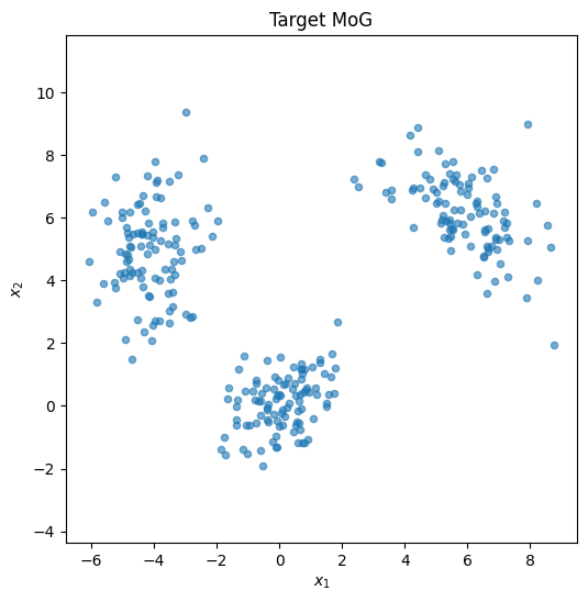
The 3-cluster MoG, seed 42, 300 points. We then train the same MLP noise predictor with the same DDPM objective.
```python theme={null}
import numpy as np
import torch
import torch.nn as nn
import torch.nn.functional as F
import matplotlib.pyplot as plt
torch.manual_seed(42)
np.random.seed(42)
device = torch.device("cuda" if torch.cuda.is_available() else "cpu")
n_samples = 300
cluster1 = np.random.multivariate_normal([0, 0], [[1, 0.5], [0.5, 1]], n_samples // 3)
cluster2 = np.random.multivariate_normal([6, 6], [[1.5, -0.7], [-0.7, 1.5]], n_samples // 3)
cluster3 = np.random.multivariate_normal([-4, 5], [[0.8, 0], [0, 2.0]], n_samples // 3)
data_np = np.vstack([cluster1, cluster2, cluster3]).astype(np.float32)
data = torch.from_numpy(data_np).to(device)
```
## Why DDIM
In the [DDPM tutorial](/aiml-common/lectures/diffusion/ddpm/ddpm_mog_tutorial) you trained a noise predictor $\epsilon_\theta(x_t, t)$ and used the **stochastic** DDPM reverse chain to generate samples. Two practical pain points come up immediately:
1. **It is slow.** DDPM samples by stepping through every timestep $T \to T-1 \to \dots \to 1$. With $T=500$ or $T=1000$ that is hundreds of network calls per sample.
2. **It is non-deterministic.** Even with a fixed initial noise $x_T$, the reverse chain injects fresh noise at each step, so you cannot reproduce a specific sample or do clean latent interpolation.
**DDIM** (Song, Meng, Ermon, 2020) addresses both with a single trick: a *non-Markovian* forward process that has the **same per-step marginals** $q(x_t \mid x_0)$ as DDPM. That means the **same trained model** $\epsilon_\theta$ can be reused, but with a different sampler that:
* Lets you skip timesteps (e.g. take 50 steps instead of 500, a 10× speedup).
* Has a tunable noise level $\eta \in [0, 1]$ where $\eta = 1$ recovers DDPM and $\eta = 0$ is fully deterministic.
The deterministic case turns the diffusion model into an invertible map between Gaussian noise and data, which is what makes things like latent-space arithmetic and image editing possible.
## Same target distribution as the DDPM tutorial
The 3-cluster MoG, seed 42, 300 points. We then train the same MLP noise predictor with the same DDPM objective.
```python theme={null}
import numpy as np
import torch
import torch.nn as nn
import torch.nn.functional as F
import matplotlib.pyplot as plt
torch.manual_seed(42)
np.random.seed(42)
device = torch.device("cuda" if torch.cuda.is_available() else "cpu")
n_samples = 300
cluster1 = np.random.multivariate_normal([0, 0], [[1, 0.5], [0.5, 1]], n_samples // 3)
cluster2 = np.random.multivariate_normal([6, 6], [[1.5, -0.7], [-0.7, 1.5]], n_samples // 3)
cluster3 = np.random.multivariate_normal([-4, 5], [[0.8, 0], [0, 2.0]], n_samples // 3)
data_np = np.vstack([cluster1, cluster2, cluster3]).astype(np.float32)
data = torch.from_numpy(data_np).to(device)
```
 ## Forward (noising) process
Same fixed Markov noising chain as DDPM: $q(x_t \mid x_0) = \mathcal{N}\!\left(x_t;\sqrt{\bar\alpha_t}\,x_0,(1-\bar\alpha_t)I\right)$. We visualize a few specific timesteps so the noise schedule is concrete before training.
```python theme={null}
T = 500
betas = torch.linspace(1e-4, 0.02, T, device=device)
alphas = 1.0 - betas
alpha_bars = torch.cumprod(alphas, dim=0)
def q_sample(x0, t, eps=None):
if eps is None:
eps = torch.randn_like(x0)
sqrt_ab = alpha_bars[t].sqrt().unsqueeze(-1)
sqrt_omab = (1 - alpha_bars[t]).sqrt().unsqueeze(-1)
return sqrt_ab * x0 + sqrt_omab * eps
```
## Forward (noising) process
Same fixed Markov noising chain as DDPM: $q(x_t \mid x_0) = \mathcal{N}\!\left(x_t;\sqrt{\bar\alpha_t}\,x_0,(1-\bar\alpha_t)I\right)$. We visualize a few specific timesteps so the noise schedule is concrete before training.
```python theme={null}
T = 500
betas = torch.linspace(1e-4, 0.02, T, device=device)
alphas = 1.0 - betas
alpha_bars = torch.cumprod(alphas, dim=0)
def q_sample(x0, t, eps=None):
if eps is None:
eps = torch.randn_like(x0)
sqrt_ab = alpha_bars[t].sqrt().unsqueeze(-1)
sqrt_omab = (1 - alpha_bars[t]).sqrt().unsqueeze(-1)
return sqrt_ab * x0 + sqrt_omab * eps
```
 ## Train the noise predictor (same architecture and objective as DDPM)
DDIM and DDPM share the **training step**, only the **sampler** differs.
```python theme={null}
class SinusoidalTimeEmbedding(nn.Module):
def __init__(self, dim):
super().__init__()
self.dim = dim
def forward(self, t):
half = self.dim // 2
freqs = torch.exp(-np.log(10000) * torch.arange(half, device=t.device) / half)
emb = t.float().unsqueeze(-1) * freqs
return torch.cat([emb.sin(), emb.cos()], dim=-1)
class NoisePredictor(nn.Module):
def __init__(self, time_dim=64, hidden=128):
super().__init__()
self.time_emb = nn.Sequential(
SinusoidalTimeEmbedding(time_dim),
nn.Linear(time_dim, time_dim), nn.SiLU(),
nn.Linear(time_dim, time_dim),
)
self.net = nn.Sequential(
nn.Linear(2 + time_dim, hidden), nn.SiLU(),
nn.Linear(hidden, hidden), nn.SiLU(),
nn.Linear(hidden, hidden), nn.SiLU(),
nn.Linear(hidden, 2),
)
def forward(self, x, t):
h = torch.cat([x, self.time_emb(t)], dim=-1)
return self.net(h)
model = NoisePredictor().to(device)
optim = torch.optim.Adam(model.parameters(), lr=1e-3)
batch_size = 256
n_steps = 4000
losses = []
for step in range(n_steps):
idx = torch.randint(0, data.shape[0], (batch_size,), device=device)
x0 = data[idx]
t = torch.randint(0, T, (batch_size,), device=device)
eps = torch.randn_like(x0)
xt = q_sample(x0, t, eps)
eps_hat = model(xt, t)
loss = F.mse_loss(eps_hat, eps)
optim.zero_grad()
loss.backward()
optim.step()
losses.append(loss.item())
if (step + 1) % 1000 == 0:
print(f"step {step + 1:>5d} loss {float(np.mean(losses[-500:])):.4f}")
print("trained.")
```
```output theme={null}
step 1000 loss 0.5713
```
```output theme={null}
step 2000 loss 0.5401
```
```output theme={null}
step 3000 loss 0.5375
```
```output theme={null}
step 4000 loss 0.5341
trained.
```
## The DDIM update rule
Given the trained $\epsilon_\theta$, define a strictly increasing sub-sequence $\tau = (\tau_1 < \tau_2 < \dots < \tau_S) \subseteq \{1, \dots, T\}$. The DDIM reverse step from $x_{\tau_i}$ to $x_{\tau_{i-1}}$ is
$x_{\tau_{i-1}} = \sqrt{\bar\alpha_{\tau_{i-1}}} \,\hat x_0 \;+\; \sqrt{1 - \bar\alpha_{\tau_{i-1}} - \sigma_{\tau_i}^2}\; \epsilon_\theta(x_{\tau_i}, \tau_i) \;+\; \sigma_{\tau_i}\, z_{\tau_i}, \quad z_{\tau_i} \sim \mathcal{N}(0, I)$
with the predicted clean sample
$\hat x_0 = \frac{x_{\tau_i} - \sqrt{1-\bar\alpha_{\tau_i}}\, \epsilon_\theta(x_{\tau_i}, \tau_i)}{\sqrt{\bar\alpha_{\tau_i}}}$
and the per-step noise scale
$\sigma_{\tau_i} \;=\; \eta \, \sqrt{\frac{1-\bar\alpha_{\tau_{i-1}}}{1-\bar\alpha_{\tau_i}}} \, \sqrt{1 - \frac{\bar\alpha_{\tau_i}}{\bar\alpha_{\tau_{i-1}}}}$
Two regimes:
* $\eta = 1$, full noise. The sampler becomes equivalent to DDPM (after accounting for sub-sequence corrections).
* $\eta = 0$, **deterministic**. The reverse step is a pure ODE-like update, $z_{\tau_i}$ disappears, and the same $x_T$ always produces the same $x_0$.
Because the model was trained on the marginals $q(x_t \mid x_0)$ (not the chain transitions), it does not care which sampler we use at inference time.
```python theme={null}
@torch.no_grad()
def ddim_sample(model, n=1000, n_steps=50, eta=0.0, x_T=None):
"""DDIM sampler.
n_steps : length of the sub-sequence tau (uniform spacing across [0, T))
eta : 0.0 = deterministic, 1.0 = stochastic (≈ DDPM)
x_T : optional fixed initial noise (for reproducibility / interpolation)
"""
if x_T is None:
x = torch.randn(n, 2, device=device)
else:
x = x_T.clone()
n = x.shape[0]
taus = torch.linspace(0, T - 1, n_steps, device=device).long()
taus = torch.unique(taus)
for i in reversed(range(len(taus))):
t_i = taus[i]
ab_i = alpha_bars[t_i]
ab_prev = alpha_bars[taus[i - 1]] if i > 0 else torch.tensor(1.0, device=device)
eps = model(x, torch.full((x.shape[0],), t_i, device=device, dtype=torch.long))
x0_hat = (x - (1 - ab_i).sqrt() * eps) / ab_i.sqrt()
sigma = eta * ((1 - ab_prev) / (1 - ab_i)).sqrt() * (1 - ab_i / ab_prev).sqrt()
dir_xt = (1 - ab_prev - sigma ** 2).clamp(min=0.0).sqrt() * eps
noise = sigma * torch.randn_like(x) if i > 0 else torch.zeros_like(x)
x = ab_prev.sqrt() * x0_hat + dir_xt + noise
return x.cpu().numpy()
```
## DDIM in 50 steps versus DDPM-equivalent in 500 steps
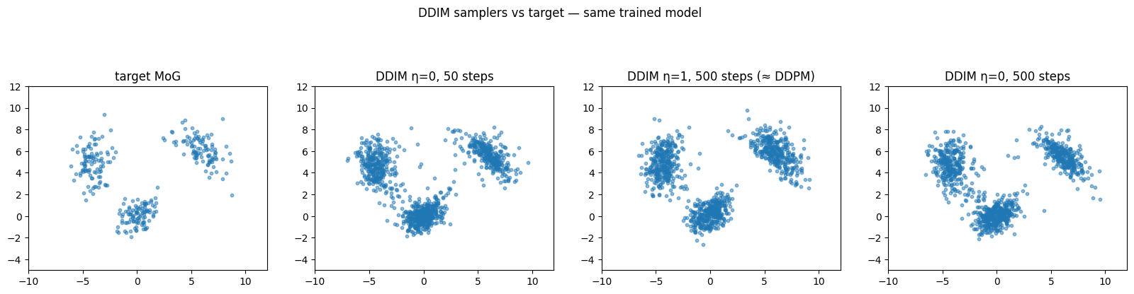
Three samplers, same model, 1000 generated points each:
* **DDIM η=0, 50 steps**, fast, deterministic.
* **DDIM η=1, 500 steps**, equivalent to DDPM, sanity check.
* **DDIM η=0, 500 steps**, deterministic with the full timestep grid.
```python theme={null}
import time
def timed(fn, *args, **kw):
if device.type == "cuda":
torch.cuda.synchronize()
start = time.time()
out = fn(*args, **kw)
if device.type == "cuda":
torch.cuda.synchronize()
return out, time.time() - start
samples_50_eta0, t_50_eta0 = timed(ddim_sample, model, n=1000, n_steps=50, eta=0.0)
samples_500_eta1, t_500_eta1 = timed(ddim_sample, model, n=1000, n_steps=500, eta=1.0)
samples_500_eta0, t_500_eta0 = timed(ddim_sample, model, n=1000, n_steps=500, eta=0.0)
print(f"DDIM eta=0, 50 steps : {t_50_eta0*1000:6.1f} ms")
print(f"DDIM eta=1, 500 steps : {t_500_eta1*1000:6.1f} ms (≈ DDPM)")
print(f"DDIM eta=0, 500 steps : {t_500_eta0*1000:6.1f} ms")
```
```output theme={null}
DDIM eta=0, 50 steps : 87.3 ms
DDIM eta=1, 500 steps : 335.1 ms (≈ DDPM)
DDIM eta=0, 500 steps : 343.1 ms
```
## Train the noise predictor (same architecture and objective as DDPM)
DDIM and DDPM share the **training step**, only the **sampler** differs.
```python theme={null}
class SinusoidalTimeEmbedding(nn.Module):
def __init__(self, dim):
super().__init__()
self.dim = dim
def forward(self, t):
half = self.dim // 2
freqs = torch.exp(-np.log(10000) * torch.arange(half, device=t.device) / half)
emb = t.float().unsqueeze(-1) * freqs
return torch.cat([emb.sin(), emb.cos()], dim=-1)
class NoisePredictor(nn.Module):
def __init__(self, time_dim=64, hidden=128):
super().__init__()
self.time_emb = nn.Sequential(
SinusoidalTimeEmbedding(time_dim),
nn.Linear(time_dim, time_dim), nn.SiLU(),
nn.Linear(time_dim, time_dim),
)
self.net = nn.Sequential(
nn.Linear(2 + time_dim, hidden), nn.SiLU(),
nn.Linear(hidden, hidden), nn.SiLU(),
nn.Linear(hidden, hidden), nn.SiLU(),
nn.Linear(hidden, 2),
)
def forward(self, x, t):
h = torch.cat([x, self.time_emb(t)], dim=-1)
return self.net(h)
model = NoisePredictor().to(device)
optim = torch.optim.Adam(model.parameters(), lr=1e-3)
batch_size = 256
n_steps = 4000
losses = []
for step in range(n_steps):
idx = torch.randint(0, data.shape[0], (batch_size,), device=device)
x0 = data[idx]
t = torch.randint(0, T, (batch_size,), device=device)
eps = torch.randn_like(x0)
xt = q_sample(x0, t, eps)
eps_hat = model(xt, t)
loss = F.mse_loss(eps_hat, eps)
optim.zero_grad()
loss.backward()
optim.step()
losses.append(loss.item())
if (step + 1) % 1000 == 0:
print(f"step {step + 1:>5d} loss {float(np.mean(losses[-500:])):.4f}")
print("trained.")
```
```output theme={null}
step 1000 loss 0.5713
```
```output theme={null}
step 2000 loss 0.5401
```
```output theme={null}
step 3000 loss 0.5375
```
```output theme={null}
step 4000 loss 0.5341
trained.
```
## The DDIM update rule
Given the trained $\epsilon_\theta$, define a strictly increasing sub-sequence $\tau = (\tau_1 < \tau_2 < \dots < \tau_S) \subseteq \{1, \dots, T\}$. The DDIM reverse step from $x_{\tau_i}$ to $x_{\tau_{i-1}}$ is
$x_{\tau_{i-1}} = \sqrt{\bar\alpha_{\tau_{i-1}}} \,\hat x_0 \;+\; \sqrt{1 - \bar\alpha_{\tau_{i-1}} - \sigma_{\tau_i}^2}\; \epsilon_\theta(x_{\tau_i}, \tau_i) \;+\; \sigma_{\tau_i}\, z_{\tau_i}, \quad z_{\tau_i} \sim \mathcal{N}(0, I)$
with the predicted clean sample
$\hat x_0 = \frac{x_{\tau_i} - \sqrt{1-\bar\alpha_{\tau_i}}\, \epsilon_\theta(x_{\tau_i}, \tau_i)}{\sqrt{\bar\alpha_{\tau_i}}}$
and the per-step noise scale
$\sigma_{\tau_i} \;=\; \eta \, \sqrt{\frac{1-\bar\alpha_{\tau_{i-1}}}{1-\bar\alpha_{\tau_i}}} \, \sqrt{1 - \frac{\bar\alpha_{\tau_i}}{\bar\alpha_{\tau_{i-1}}}}$
Two regimes:
* $\eta = 1$, full noise. The sampler becomes equivalent to DDPM (after accounting for sub-sequence corrections).
* $\eta = 0$, **deterministic**. The reverse step is a pure ODE-like update, $z_{\tau_i}$ disappears, and the same $x_T$ always produces the same $x_0$.
Because the model was trained on the marginals $q(x_t \mid x_0)$ (not the chain transitions), it does not care which sampler we use at inference time.
```python theme={null}
@torch.no_grad()
def ddim_sample(model, n=1000, n_steps=50, eta=0.0, x_T=None):
"""DDIM sampler.
n_steps : length of the sub-sequence tau (uniform spacing across [0, T))
eta : 0.0 = deterministic, 1.0 = stochastic (≈ DDPM)
x_T : optional fixed initial noise (for reproducibility / interpolation)
"""
if x_T is None:
x = torch.randn(n, 2, device=device)
else:
x = x_T.clone()
n = x.shape[0]
taus = torch.linspace(0, T - 1, n_steps, device=device).long()
taus = torch.unique(taus)
for i in reversed(range(len(taus))):
t_i = taus[i]
ab_i = alpha_bars[t_i]
ab_prev = alpha_bars[taus[i - 1]] if i > 0 else torch.tensor(1.0, device=device)
eps = model(x, torch.full((x.shape[0],), t_i, device=device, dtype=torch.long))
x0_hat = (x - (1 - ab_i).sqrt() * eps) / ab_i.sqrt()
sigma = eta * ((1 - ab_prev) / (1 - ab_i)).sqrt() * (1 - ab_i / ab_prev).sqrt()
dir_xt = (1 - ab_prev - sigma ** 2).clamp(min=0.0).sqrt() * eps
noise = sigma * torch.randn_like(x) if i > 0 else torch.zeros_like(x)
x = ab_prev.sqrt() * x0_hat + dir_xt + noise
return x.cpu().numpy()
```
## DDIM in 50 steps versus DDPM-equivalent in 500 steps
Three samplers, same model, 1000 generated points each:
* **DDIM η=0, 50 steps**, fast, deterministic.
* **DDIM η=1, 500 steps**, equivalent to DDPM, sanity check.
* **DDIM η=0, 500 steps**, deterministic with the full timestep grid.
```python theme={null}
import time
def timed(fn, *args, **kw):
if device.type == "cuda":
torch.cuda.synchronize()
start = time.time()
out = fn(*args, **kw)
if device.type == "cuda":
torch.cuda.synchronize()
return out, time.time() - start
samples_50_eta0, t_50_eta0 = timed(ddim_sample, model, n=1000, n_steps=50, eta=0.0)
samples_500_eta1, t_500_eta1 = timed(ddim_sample, model, n=1000, n_steps=500, eta=1.0)
samples_500_eta0, t_500_eta0 = timed(ddim_sample, model, n=1000, n_steps=500, eta=0.0)
print(f"DDIM eta=0, 50 steps : {t_50_eta0*1000:6.1f} ms")
print(f"DDIM eta=1, 500 steps : {t_500_eta1*1000:6.1f} ms (≈ DDPM)")
print(f"DDIM eta=0, 500 steps : {t_500_eta0*1000:6.1f} ms")
```
```output theme={null}
DDIM eta=0, 50 steps : 87.3 ms
DDIM eta=1, 500 steps : 335.1 ms (≈ DDPM)
DDIM eta=0, 500 steps : 343.1 ms
```
 ## Determinism: same noise, same sample
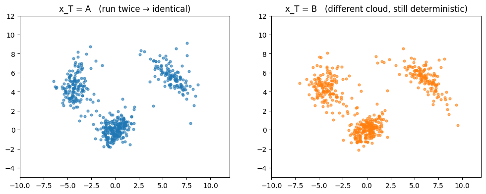
With $\eta = 0$ the sampler is a deterministic function of the initial noise $x_T$. Run it twice with the same $x_T$ and you get bit-identical outputs, regardless of how many steps you take.
```python theme={null}
x_T = torch.randn(500, 2, device=device)
out_a = ddim_sample(model, n_steps=50, eta=0.0, x_T=x_T)
out_b = ddim_sample(model, n_steps=50, eta=0.0, x_T=x_T)
max_abs_diff = float(np.max(np.abs(out_a - out_b)))
print(f"max |x_a - x_b| = {max_abs_diff:.3e} (should be 0 with eta=0)")
x_T2 = torch.randn(500, 2, device=device)
out_c = ddim_sample(model, n_steps=50, eta=0.0, x_T=x_T2)
```
```output theme={null}
max |x_a - x_b| = 0.000e+00 (should be 0 with eta=0)
```
## Determinism: same noise, same sample
With $\eta = 0$ the sampler is a deterministic function of the initial noise $x_T$. Run it twice with the same $x_T$ and you get bit-identical outputs, regardless of how many steps you take.
```python theme={null}
x_T = torch.randn(500, 2, device=device)
out_a = ddim_sample(model, n_steps=50, eta=0.0, x_T=x_T)
out_b = ddim_sample(model, n_steps=50, eta=0.0, x_T=x_T)
max_abs_diff = float(np.max(np.abs(out_a - out_b)))
print(f"max |x_a - x_b| = {max_abs_diff:.3e} (should be 0 with eta=0)")
x_T2 = torch.randn(500, 2, device=device)
out_c = ddim_sample(model, n_steps=50, eta=0.0, x_T=x_T2)
```
```output theme={null}
max |x_a - x_b| = 0.000e+00 (should be 0 with eta=0)
```
 ## Latent interpolation: slerp on $x_T$
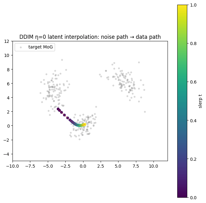
Because $\eta = 0$ DDIM is a deterministic invertible map, you can pick two endpoints in noise space and walk a path between them; each intermediate noise decodes to a coherent point in data space. The right path on the unit sphere is **spherical linear interpolation** (slerp), which preserves the Gaussian magnitude.
```python theme={null}
def slerp(z0, z1, t):
"""Spherical linear interpolation in 2D Gaussian noise space."""
z0_n = z0 / z0.norm()
z1_n = z1 / z1.norm()
omega = torch.acos((z0_n * z1_n).sum().clamp(-1.0, 1.0))
so = torch.sin(omega)
return (torch.sin((1 - t) * omega) / so) * z0 + (torch.sin(t * omega) / so) * z1
torch.manual_seed(0)
z_a = torch.randn(2, device=device)
z_b = torch.randn(2, device=device)
n_path = 50
ts = torch.linspace(0, 1, n_path)
path = torch.stack([slerp(z_a, z_b, float(t)) for t in ts], dim=0).to(device)
decoded = ddim_sample(model, n_steps=50, eta=0.0, x_T=path)
```
## Latent interpolation: slerp on $x_T$
Because $\eta = 0$ DDIM is a deterministic invertible map, you can pick two endpoints in noise space and walk a path between them; each intermediate noise decodes to a coherent point in data space. The right path on the unit sphere is **spherical linear interpolation** (slerp), which preserves the Gaussian magnitude.
```python theme={null}
def slerp(z0, z1, t):
"""Spherical linear interpolation in 2D Gaussian noise space."""
z0_n = z0 / z0.norm()
z1_n = z1 / z1.norm()
omega = torch.acos((z0_n * z1_n).sum().clamp(-1.0, 1.0))
so = torch.sin(omega)
return (torch.sin((1 - t) * omega) / so) * z0 + (torch.sin(t * omega) / so) * z1
torch.manual_seed(0)
z_a = torch.randn(2, device=device)
z_b = torch.randn(2, device=device)
n_path = 50
ts = torch.linspace(0, 1, n_path)
path = torch.stack([slerp(z_a, z_b, float(t)) for t in ts], dim=0).to(device)
decoded = ddim_sample(model, n_steps=50, eta=0.0, x_T=path)
```
 ## Connections to other concepts
* **Sampler decoupling.** Training trains; sampling samples. DDIM proves you can swap samplers freely as long as marginals are preserved. Modern stacks ship many samplers (DDIM, DPM-Solver, Euler, Heun, …) on top of the *same* DDPM-trained network.
* **Step count is a knob, not a constant.** Image-generation pipelines routinely use 20-50 DDIM steps in production where DDPM would take 1000.
* **Deterministic = invertible.** $\eta = 0$ DDIM gives you a noise-to-data map you can run forwards and backwards, enabling editing and interpolation.
* **Bridge to flows and ODEs.** Deterministic DDIM is the discretization of a probability-flow ODE. That connection underlies most of the recent diffusion-model speedup work (consistency models, rectified flow, …).
* **Score-based unification.** The [Score MoG Tutorial](/aiml-common/lectures/diffusion/score-based/score-mog-example/score_mog_example) makes that ODE bridge concrete: train $s_\theta(x, \sigma)$ on the same MoG, then sample via annealed Langevin or the reverse-time SDE. Deterministic DDIM is the probability-flow ODE limit of that score-SDE.
## References
1. Song, Meng, Ermon. *Denoising Diffusion Implicit Models.* ICLR 2021. [arxiv.org/abs/2010.02502](https://arxiv.org/abs/2010.02502)
2. Ho, Jain, Abbeel. *Denoising Diffusion Probabilistic Models.* NeurIPS 2020. [arxiv.org/abs/2006.11239](https://arxiv.org/abs/2006.11239)
3. Song et al. *Score-Based Generative Modeling through Stochastic Differential Equations.* ICLR 2021. [arxiv.org/abs/2011.13456](https://arxiv.org/abs/2011.13456)
## PyTorch reference
| PyTorch class | Description |
| ---------------------------------------------------------------------------------------- | ----------------------------------------------------------------------------- |
| [`nn.Sequential`](https://docs.pytorch.org/docs/2.12/generated/torch.nn.Sequential.html) | A sequential container. |
| [`nn.Linear`](https://docs.pytorch.org/docs/2.12/generated/torch.nn.Linear.html) | Applies an affine linear transformation to the incoming data: $y = xA^T + b$. |
| [`nn.SiLU`](https://docs.pytorch.org/docs/2.12/generated/torch.nn.SiLU.html) | Applies the Sigmoid Linear Unit (SiLU) function, element-wise. |
***
[Edit this page on GitHub](https://github.com/aegean-ai/eaia/edit/main/src/aiml-common/lectures/diffusion/ddim/ddim_mog_tutorial.mdx) or [file an issue](https://github.com/aegean-ai/eaia/issues/new/choose).
## Connections to other concepts
* **Sampler decoupling.** Training trains; sampling samples. DDIM proves you can swap samplers freely as long as marginals are preserved. Modern stacks ship many samplers (DDIM, DPM-Solver, Euler, Heun, …) on top of the *same* DDPM-trained network.
* **Step count is a knob, not a constant.** Image-generation pipelines routinely use 20-50 DDIM steps in production where DDPM would take 1000.
* **Deterministic = invertible.** $\eta = 0$ DDIM gives you a noise-to-data map you can run forwards and backwards, enabling editing and interpolation.
* **Bridge to flows and ODEs.** Deterministic DDIM is the discretization of a probability-flow ODE. That connection underlies most of the recent diffusion-model speedup work (consistency models, rectified flow, …).
* **Score-based unification.** The [Score MoG Tutorial](/aiml-common/lectures/diffusion/score-based/score-mog-example/score_mog_example) makes that ODE bridge concrete: train $s_\theta(x, \sigma)$ on the same MoG, then sample via annealed Langevin or the reverse-time SDE. Deterministic DDIM is the probability-flow ODE limit of that score-SDE.
## References
1. Song, Meng, Ermon. *Denoising Diffusion Implicit Models.* ICLR 2021. [arxiv.org/abs/2010.02502](https://arxiv.org/abs/2010.02502)
2. Ho, Jain, Abbeel. *Denoising Diffusion Probabilistic Models.* NeurIPS 2020. [arxiv.org/abs/2006.11239](https://arxiv.org/abs/2006.11239)
3. Song et al. *Score-Based Generative Modeling through Stochastic Differential Equations.* ICLR 2021. [arxiv.org/abs/2011.13456](https://arxiv.org/abs/2011.13456)
## PyTorch reference
| PyTorch class | Description |
| ---------------------------------------------------------------------------------------- | ----------------------------------------------------------------------------- |
| [`nn.Sequential`](https://docs.pytorch.org/docs/2.12/generated/torch.nn.Sequential.html) | A sequential container. |
| [`nn.Linear`](https://docs.pytorch.org/docs/2.12/generated/torch.nn.Linear.html) | Applies an affine linear transformation to the incoming data: $y = xA^T + b$. |
| [`nn.SiLU`](https://docs.pytorch.org/docs/2.12/generated/torch.nn.SiLU.html) | Applies the Sigmoid Linear Unit (SiLU) function, element-wise. |
***
[Edit this page on GitHub](https://github.com/aegean-ai/eaia/edit/main/src/aiml-common/lectures/diffusion/ddim/ddim_mog_tutorial.mdx) or [file an issue](https://github.com/aegean-ai/eaia/issues/new/choose).