> ## Documentation Index
> Fetch the complete documentation index at: https://aegean.ai/llms.txt
> Use this file to discover all available pages before exploring further.
# Denoising Diffusion Probabilistic Models
> Forward and reverse processes, three-step worked example, and the VAE-ELBO derivation of the DDPM training loss.
## Diffusion models at a glance
A denoising diffusion model is built from two coupled Markov chains running in opposite directions over the same set of intermediate states $x_0, x_1, \ldots, x_T$:
* **Forward diffusion process** (fixed). Gradually corrupts a clean data point $x_0$ into pure Gaussian noise $x_T$ by adding a small amount of Gaussian noise at each step. No learned parameters; specified entirely by a noise schedule $\beta_t$. Read it as a stack of **fixed VAE encoders**.
* **Reverse denoising process** (learnable). Starts from pure noise $x_T \sim \mathcal{N}(\mathbf{0}, \mathbf{I})$ and gradually denoises down to $x_0$. Read it as a stack of **learnable VAE decoders** — but with a single neural network shared across all $T$ timesteps and conditioned on $t$.
Pictorially, both chains run over the same intermediate states:
**Forward q (fixed): gradually add noise**
 *Editable Mermaid source: [`images/forward-chain.mermaid.md`](images/forward-chain.mermaid.md)*
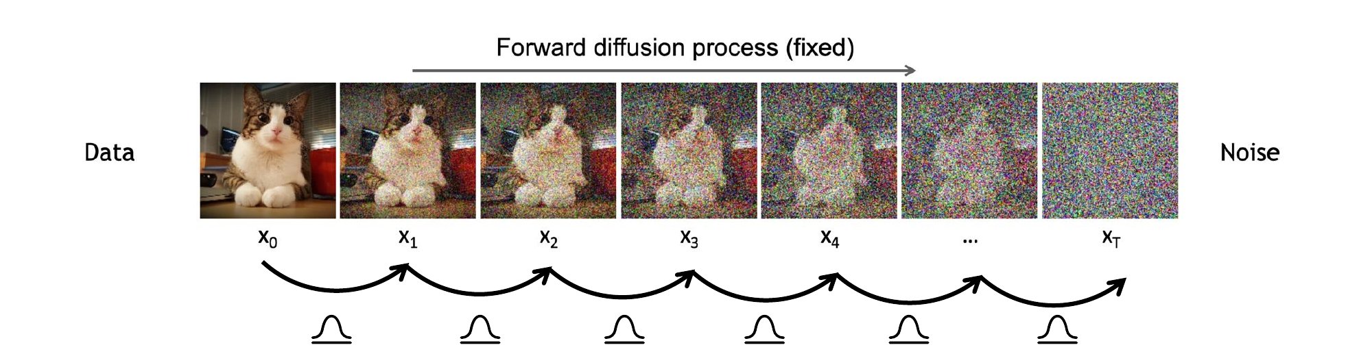 *Filmstrip from [CMU 11-785, Lecture 24 (Diffusion)](https://deeplearning.cs.cmu.edu/F24/document/slides/lec24.diffusion.pdf), slide 24.*
**Reverse pθ (learned): gradually denoise**
*Filmstrip from [CMU 11-785, Lecture 24 (Diffusion)](https://deeplearning.cs.cmu.edu/F24/document/slides/lec24.diffusion.pdf), slide 24.*
**Reverse pθ (learned): gradually denoise**
 *Editable Mermaid source: [`images/reverse-chain.mermaid.md`](images/reverse-chain.mermaid.md)*
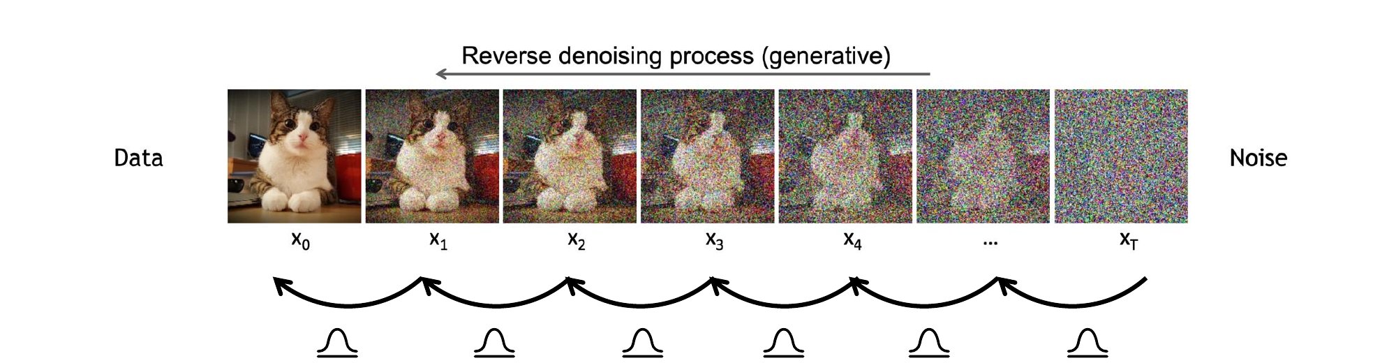 *Filmstrip from [CMU 11-785, Lecture 24 (Diffusion)](https://deeplearning.cs.cmu.edu/F24/document/slides/lec24.diffusion.pdf), slide 27.*
Generation = run the reverse chain. Training = teach the reverse chain to undo a step of the forward chain. The rest of this page builds both chains from a single mathematical primitive: Bishop's linear-Gaussian theorem.
## Bishop's linear-Gaussian theorem applied to one diffusion step
A single noising step couples $x_{t-1}$ and $x_t$ through a linear-Gaussian relationship, an instance of [Bishop's linear-Gaussian theorem](/aiml-common/lectures/ml-math/probability/gaussians/gaussians#bishop-s-linear-gaussian-theorem) on the gaussians prerequisite page. Recognizing the kernel as a special case of Bishop's template lets us read off the marginal in closed form and gives a clean route to the multi-step closed-form jump $q(x_t \mid x_0)$ in the next section.
Specialize the theorem to one DDPM step. Take $x = x_{t-1}$, $y = x_t$, with prior $x_{t-1} \sim \mathcal{N}(\mu_{t-1}, \Sigma_{t-1})$. The **forward kernel** is the linear-Gaussian conditional
$$
q(x_t \mid x_{t-1}) = \mathcal{N}\left(x_t \mid \sqrt{1-\beta_t}\, x_{t-1},\; \beta_t I\right),
$$
which matches Bishop's $\mathbf{y} = \mathbf{A}\mathbf{x} + \mathbf{b} + \boldsymbol{\varepsilon}$ template with $\mathbf{A} = \sqrt{1-\beta_t}\, I$, $\mathbf{b} = 0$, conditional precision $\mathbf{L} = \beta_t^{-1} I$, and prior precision $\boldsymbol{\Lambda} = \Sigma_{t-1}^{-1}$. Plugging into Bishop's marginal formula gives the **forward marginal**
$$
q(x_t) = \mathcal{N}\left(x_t \mid \sqrt{1-\beta_t}\, \mu_{t-1},\; \beta_t I + (1-\beta_t)\, \Sigma_{t-1}\right).
$$
This is the workhorse. Every later result composes the forward kernel: the full forward chain $q(x_{1:T} \mid x_0)$, the closed-form one-shot jump $q(x_t \mid x_0)$, and the **forward posterior** $q(x_{t-1} \mid x_t, x_0)$ that turns out to be the right reverse-direction target — exact in closed form for any data distribution, and the object the learned $p_\theta$ will be trained to imitate. The next two sections build out the forward chain; after that the learned $p_\theta$ is introduced.
## The forward process: composing $T$ steps
The single-step kernel $q(x_t \mid x_{t-1})$, repeated $t$ times with a fixed schedule $\beta_1, \ldots, \beta_T \in (0, 1)$, defines the full forward chain:
$$
q(x_{1:T} \mid x_0) \;=\; \prod_{t=1}^{T} q(x_t \mid x_{t-1}).
$$
**Closed-form jump from $x_0$ to any $x_t$.** Because each step is linear-Gaussian and they compose, you can sample $x_t$ in a single shot without simulating the intermediate states. Define $\alpha_t = 1 - \beta_t$ and the cumulative product $\bar\alpha_t = \prod_{s=1}^t \alpha_s$. Iterating Bishop's per-step recursion across $t$ steps gives
$$
\begin{aligned}
q(x_t \mid x_0) &= \mathcal{N}\!\left(x_t;\; \sqrt{\bar\alpha_t}\, x_0,\; (1 - \bar\alpha_t)\, \mathbf{I}\right), \\
x_t &= \sqrt{\bar\alpha_t}\, x_0 \;+\; \sqrt{1 - \bar\alpha_t}\,\epsilon, \quad \epsilon \sim \mathcal{N}(\mathbf{0}, \mathbf{I}).
\end{aligned}
$$
This identity is what makes DDPM training cheap: at every gradient step you draw a random $t$ and compute $x_t$ directly from $x_0$ rather than rolling out the chain.
The schedule is designed so that $\bar\alpha_T \to 0$, which makes $q(x_T \mid x_0) \approx \mathcal{N}(\mathbf{0}, \mathbf{I})$ regardless of $x_0$. The endpoint of the forward chain is therefore (approximately) data-independent pure noise — the same prior the reverse chain will start from.
## The reverse process: parameterizing what $q$ hides
To generate, we want to draw $x_T \sim \mathcal{N}(\mathbf{0}, \mathbf{I})$ and then iteratively sample
$$
x_{t-1} \;\sim\; q(x_{t-1} \mid x_t), \qquad t = T, T-1, \ldots, 1.
$$
The catch: $q(x_{t-1} \mid x_t)$ as a function of $x_t$ alone is **not directly tractable** at sampling time. Even though $x_{t-1}$ and $x_t$ are jointly distributed under the forward joint, computing this conditional requires marginalizing over the data distribution $q(x_0)$ — which is precisely what we are trying to model.
DDPM's modeling choice: approximate the reverse step with a learned Gaussian,
$$
p_\theta(x_{t-1} \mid x_t) \;=\; \mathcal{N}\!\left(x_{t-1};\; \mu_\theta(x_t, t),\; \sigma_t^2\, \mathbf{I}\right).
$$
Two reasons this functional form is reasonable:
1. **Small-$\beta_t$ limit.** When each forward step injects only a little noise, the true reverse conditional $q(x_{t-1} \mid x_t)$ — even with a non-Gaussian data distribution — is well-approximated by a Gaussian (Sohl-Dickstein et al. 2015). That is the local justification for choosing a Gaussian functional form for $p_\theta$.
2. **Conditioned on $x_0$, $q$ is genuinely Gaussian.** A close cousin, $q(x_{t-1} \mid x_t, x_0)$, is exactly Gaussian for *any* data distribution $q(x_0)$ — Bayes' rule on the forward joint with $x_0$ as a fixed parameter (full derivation in the [Notes on the reverse conditional](#notes-on-the-reverse-conditional) deep-dive below). Training will use this two-conditional form (which has $x_0$ available) as the *target* the learned $p_\theta$ should match.
Two notes on the parameters:
* $\mu_\theta(x_t, t)$ is the only **learned** quantity. A single neural network produces it for every $t$, with $t$ fed in through a sinusoidal **time embedding** so the same weights handle every noise level.
* $\sigma_t^2$ is typically **fixed** by the schedule, commonly either $\beta_t$ or the DDPM posterior variance $\tilde\beta_t$ from $q(x_{t-1} \mid x_t, x_0)$, so the variance is not learned in the basic DDPM.
The full reverse joint factorizes as
$$
p_\theta(x_{0:T}) \;=\; p(x_T)\, \prod_{t=1}^{T} p_\theta(x_{t-1} \mid x_t),
\qquad
p(x_T) = \mathcal{N}(\mathbf{0}, \mathbf{I}),
$$
and sampling is the obvious thing: draw $x_T$ from the standard Gaussian, then walk one step at a time toward $x_0$.
## Notes on the reverse conditional
With both chains in place, three observations are worth flagging — one notational, two structural. The deep-dive at the end is safe to skip on a first reading.
1. **Notation: what $q$ does and does not mean.** The symbol $q$ does *not* tag a direction in time. The forward process defines a joint distribution $q(x_0, x_1, \ldots, x_T) = q(x_0) \prod_{t=1}^{T} q(x_t \mid x_{t-1})$, and **anything** you can compute from that joint stays inside the q-family. Both $q(x_t \mid x_{t-1})$ and its time-reversal $q(x_{t-1} \mid x_t)$ live in it. But only some of these conditionals stay analytically simple after marginalizing over the data distribution: $q(x_t \mid x_{t-1})$ is fixed and explicit by construction, while $q(x_{t-1} \mid x_t)$ is generally not available in closed form unless extra Gaussian assumptions are imposed. The contrast is with $p_\theta(x_{t-1} \mid x_t)$, which is the **learned** generative model used at sampling time, where $x_0$ (and therefore the data distribution) is no longer available.
2. **What $p_\theta$ targets.** The training target the learned $p_\theta(x_{t-1} \mid x_t)$ is fitted against is the **forward posterior** $q(x_{t-1} \mid x_t, x_0)$, which is exactly Gaussian for any data distribution (see the deep-dive below). At sampling time $x_0$ is unavailable, so the network's job is to predict what that posterior would have said using only $x_t$ and $t$.
3. **Variance accumulates predictably.** Each forward step adds $\beta_t I$ to a $(1-\beta_t)$-shrunken copy of $\Sigma_{t-1}$. The closed-form jump $q(x_t \mid x_0) = \mathcal{N}(\sqrt{\bar\alpha_t}\, x_0,\, (1 - \bar\alpha_t)\, I)$ in the forward-process section is precisely the iteration of this rule across $T$ steps.
The naive reverse conditional $q(x_{t-1} \mid x_t)$ — conditioning only on the current noisy state — is **not** in closed form for an arbitrary data distribution: it requires marginalizing over $q(x_0)$, which is exactly what we are trying to model. The standard DDPM derivation (Ho et al. 2020, eq. 6-7) sidesteps that by working with $q(x_{t-1} \mid x_t, x_0)$ — conditioning on **both** the current noisy state *and* the original clean sample — which is exactly Gaussian for *any* $q(x_0)$.
The two-conditional form is Gaussian for *any* data distribution $q(x_0)$. Apply Bayes' rule on the forward joint:
$$
q(x_{t-1} \mid x_t, x_0) \;=\; \frac{q(x_t \mid x_{t-1}, x_0)\, q(x_{t-1} \mid x_0)}{q(x_t \mid x_0)}.
$$
By the Markov property of the forward chain, $q(x_t \mid x_{t-1}, x_0) = q(x_t \mid x_{t-1})$ is the Gaussian noising kernel. The other two terms are the closed-form jumps from $x_0$ derived in the forward-process section, both Gaussian. The product/quotient of three Gaussians (in $x_{t-1}$) is again Gaussian. The data distribution $q(x_0)$ never enters because **$x_0$ is a fixed parameter here, not a random variable being marginalized over** — its value just shifts the means.
By contrast, $q(x_{t-1} \mid x_t)$ without $x_0$ marginalizes $x_0$ out:
$$
q(x_{t-1} \mid x_t) \;=\; \int q(x_{t-1} \mid x_t, x_0)\, q(x_0 \mid x_t)\, dx_0,
$$
a mixture of Gaussians weighted by the posterior $q(x_0 \mid x_t)$, generally non-Gaussian unless $q(x_0)$ itself is Gaussian. The two-conditional form $q(x_{t-1} \mid x_t, x_0)$ avoids this entirely: with $x_0$ as a fixed parameter, the data distribution drops out of the algebra and the closed form holds regardless of $q(x_0)$. That is the **forward posterior** that appears in the ELBO derivation below — at training time you have $x_0$ available, and the result is a Gaussian whose mean and variance are explicit functions of $(x_t, x_0, t)$ alone.
Consider a toy diffusion model with only three noising steps:
$$
x_0 \;\to\; x_1 \;\to\; x_2 \;\to\; x_3.
$$
$x_0$ is a clean data sample (for example, an image) and $x_3$ is almost Gaussian noise. Pick a forward noise schedule
$$
\beta_1, \beta_2, \beta_3 \in (0, 1),
$$
and define $\alpha_t = 1 - \beta_t$ together with the cumulative product
$$
\bar\alpha_t = \prod_{s=1}^{t} \alpha_s,
\qquad\text{so}\qquad
\bar\alpha_1 = \alpha_1,\quad
\bar\alpha_2 = \alpha_1 \alpha_2,\quad
\bar\alpha_3 = \alpha_1 \alpha_2 \alpha_3.
$$
**Forward process.** The forward process is fixed: it gradually corrupts the data by
$$
q(x_t \mid x_{t-1}) = \mathcal{N}\left(x_t;\; \sqrt{\alpha_t}\, x_{t-1},\; \beta_t I\right).
$$
For the three steps,
$$
q(x_1 \mid x_0) = \mathcal{N}\left(x_1;\; \sqrt{\alpha_1}\, x_0,\; \beta_1 I\right),
$$
$$
q(x_2 \mid x_1) = \mathcal{N}\left(x_2;\; \sqrt{\alpha_2}\, x_1,\; \beta_2 I\right),
$$
$$
q(x_3 \mid x_2) = \mathcal{N}\left(x_3;\; \sqrt{\alpha_3}\, x_2,\; \beta_3 I\right).
$$
Equivalently, you can sample any noisy point directly from $x_0$:
$$
q(x_t \mid x_0) = \mathcal{N}\left(x_t;\; \sqrt{\bar\alpha_t}\, x_0,\; (1 - \bar\alpha_t)\, I\right),
$$
so the final noisy sample is
$$
x_3 = \sqrt{\bar\alpha_3}\, x_0 + \sqrt{1 - \bar\alpha_3}\, \epsilon,
\qquad \epsilon \sim \mathcal{N}(0, I).
$$
**Reverse process.** The reverse process tries to undo the corruption: $x_3 \to x_2 \to x_1 \to x_0$. Parameterize the learned reverse kernel as
$$
p_\theta(x_{t-1} \mid x_t) = \mathcal{N}\left(x_{t-1};\; \mu_\theta(x_t),\; \Sigma_\theta(x_t)\right),
$$
instantiated at the three steps as $p_\theta(x_2 \mid x_3)$, $p_\theta(x_1 \mid x_2)$, $p_\theta(x_0 \mid x_1)$.
A note on notation: $\mu_\theta(x_t)$ and $\epsilon_\theta(x_t)$ are written with a single argument because $t$ is already pinned down by the subscript on $x_t$. In code, $\mu_\theta$ and $\epsilon_\theta$ are a *single* shared network used at every timestep, conditioned on $t$ through a learned time embedding; the $t$ argument is implicit in the input typing.
In DDPM the network predicts the noise $\epsilon_\theta(x_t)$ that was added. Plugging that into the reverse mean gives
$$
\mu_\theta(x_t) = \frac{1}{\sqrt{\alpha_t}}\left( x_t - \frac{\beta_t}{\sqrt{1 - \bar\alpha_t}}\, \epsilon_\theta(x_t) \right).
$$
Starting from $x_3 \sim \mathcal{N}(0, I)$, the three reverse transitions are
$$
\mu_\theta(x_3) = \frac{1}{\sqrt{\alpha_3}}\left( x_3 - \frac{\beta_3}{\sqrt{1 - \bar\alpha_3}}\, \epsilon_\theta(x_3) \right),
\qquad
x_2 \sim \mathcal{N}\left(\mu_\theta(x_3),\; \Sigma_\theta(x_3)\right),
$$
$$
\mu_\theta(x_2) = \frac{1}{\sqrt{\alpha_2}}\left( x_2 - \frac{\beta_2}{\sqrt{1 - \bar\alpha_2}}\, \epsilon_\theta(x_2) \right),
\qquad
x_1 \sim \mathcal{N}\left(\mu_\theta(x_2),\; \Sigma_\theta(x_2)\right),
$$
$$
\mu_\theta(x_1) = \frac{1}{\sqrt{\alpha_1}}\left( x_1 - \frac{\beta_1}{\sqrt{1 - \bar\alpha_1}}\, \epsilon_\theta(x_1) \right),
\qquad
x_0 \sim \mathcal{N}\left(\mu_\theta(x_1),\; \Sigma_\theta(x_1)\right).
$$
The essential idea: the forward chain adds known Gaussian noise, and the reverse chain learns how much noise to remove. Putting both directions on the same picture,
$$
x_0 \xrightarrow{q} x_1 \xrightarrow{q} x_2 \xrightarrow{q} x_3,
\qquad
x_3 \sim \mathcal{N}(0, I) \xrightarrow{p_\theta} x_2 \xrightarrow{p_\theta} x_1 \xrightarrow{p_\theta} x_0.
$$
## What the network outputs
The reverse-step distribution is parameterized as
$$
p_\theta(x_{t-1} \mid x_t) = \mathcal{N}\!\left(x_{t-1};\, \mu_\theta(x_t, t),\, \sigma_t^2\, \mathbf{I}\right),
$$
but what the neural network *literally computes* is a design choice. There are three algebraically equivalent options:
1. **Predict the mean directly** — $\mu_\theta(x_t, t)$. The most direct read of the parameterization above; the network output is a vector with the shape of $x_t$, used as the mean of the reverse Gaussian.
2. **Predict the noise** — $\epsilon_\theta(x_t, t)$. The network outputs a vector with the shape of $x_t$ that estimates the noise that was added when forming $x_t$ from $x_0$ via the closed-form jump. The reverse-step mean is then derived analytically:
$$
\mu_\theta(x_t, t) = \frac{1}{\sqrt{\alpha_t}}\!\left( x_t - \frac{\beta_t}{\sqrt{1 - \bar\alpha_t}}\, \epsilon_\theta(x_t, t) \right).
$$
3. **Predict the clean data** — $\hat{x}_{0,\theta}(x_t, t)$. The network outputs an estimate of the original $x_0$. The reverse-step mean is derived from the forward posterior $q(x_{t-1} \mid x_t, x_0)$ with the network's $\hat{x}_0$ plugged in for the unknown $x_0$.
These three are interchangeable under the reparameterization $x_t = \sqrt{\bar\alpha_t}\, x_0 + \sqrt{1 - \bar\alpha_t}\, \epsilon$:
* Given $(x_t, \hat\epsilon)$: solve for $\hat{x}_0 = (x_t - \sqrt{1 - \bar\alpha_t}\, \hat\epsilon) \,/\, \sqrt{\bar\alpha_t}$.
* Given $(x_t, \hat{x}_0)$: solve for $\hat\epsilon = (x_t - \sqrt{\bar\alpha_t}\, \hat{x}_0) \,/\, \sqrt{1 - \bar\alpha_t}$.
**DDPM picks ε-prediction.** Three reasons make it empirically dominant:
* The training target $\epsilon \sim \mathcal{N}(\mathbf{0}, \mathbf{I})$ has fixed scale at every $t$, so the regression problem is well-conditioned across all noise levels.
* The corresponding training loss collapses to a plain unweighted MSE — the $L_\text{simple}$ derived in the next section.
* The network's job becomes a single intuitive task: "look at this noisy data and tell me the noise that was added".
Concretely, one forward pass of the DDPM network looks like:
*Filmstrip from [CMU 11-785, Lecture 24 (Diffusion)](https://deeplearning.cs.cmu.edu/F24/document/slides/lec24.diffusion.pdf), slide 27.*
Generation = run the reverse chain. Training = teach the reverse chain to undo a step of the forward chain. The rest of this page builds both chains from a single mathematical primitive: Bishop's linear-Gaussian theorem.
## Bishop's linear-Gaussian theorem applied to one diffusion step
A single noising step couples $x_{t-1}$ and $x_t$ through a linear-Gaussian relationship, an instance of [Bishop's linear-Gaussian theorem](/aiml-common/lectures/ml-math/probability/gaussians/gaussians#bishop-s-linear-gaussian-theorem) on the gaussians prerequisite page. Recognizing the kernel as a special case of Bishop's template lets us read off the marginal in closed form and gives a clean route to the multi-step closed-form jump $q(x_t \mid x_0)$ in the next section.
Specialize the theorem to one DDPM step. Take $x = x_{t-1}$, $y = x_t$, with prior $x_{t-1} \sim \mathcal{N}(\mu_{t-1}, \Sigma_{t-1})$. The **forward kernel** is the linear-Gaussian conditional
$$
q(x_t \mid x_{t-1}) = \mathcal{N}\left(x_t \mid \sqrt{1-\beta_t}\, x_{t-1},\; \beta_t I\right),
$$
which matches Bishop's $\mathbf{y} = \mathbf{A}\mathbf{x} + \mathbf{b} + \boldsymbol{\varepsilon}$ template with $\mathbf{A} = \sqrt{1-\beta_t}\, I$, $\mathbf{b} = 0$, conditional precision $\mathbf{L} = \beta_t^{-1} I$, and prior precision $\boldsymbol{\Lambda} = \Sigma_{t-1}^{-1}$. Plugging into Bishop's marginal formula gives the **forward marginal**
$$
q(x_t) = \mathcal{N}\left(x_t \mid \sqrt{1-\beta_t}\, \mu_{t-1},\; \beta_t I + (1-\beta_t)\, \Sigma_{t-1}\right).
$$
This is the workhorse. Every later result composes the forward kernel: the full forward chain $q(x_{1:T} \mid x_0)$, the closed-form one-shot jump $q(x_t \mid x_0)$, and the **forward posterior** $q(x_{t-1} \mid x_t, x_0)$ that turns out to be the right reverse-direction target — exact in closed form for any data distribution, and the object the learned $p_\theta$ will be trained to imitate. The next two sections build out the forward chain; after that the learned $p_\theta$ is introduced.
## The forward process: composing $T$ steps
The single-step kernel $q(x_t \mid x_{t-1})$, repeated $t$ times with a fixed schedule $\beta_1, \ldots, \beta_T \in (0, 1)$, defines the full forward chain:
$$
q(x_{1:T} \mid x_0) \;=\; \prod_{t=1}^{T} q(x_t \mid x_{t-1}).
$$
**Closed-form jump from $x_0$ to any $x_t$.** Because each step is linear-Gaussian and they compose, you can sample $x_t$ in a single shot without simulating the intermediate states. Define $\alpha_t = 1 - \beta_t$ and the cumulative product $\bar\alpha_t = \prod_{s=1}^t \alpha_s$. Iterating Bishop's per-step recursion across $t$ steps gives
$$
\begin{aligned}
q(x_t \mid x_0) &= \mathcal{N}\!\left(x_t;\; \sqrt{\bar\alpha_t}\, x_0,\; (1 - \bar\alpha_t)\, \mathbf{I}\right), \\
x_t &= \sqrt{\bar\alpha_t}\, x_0 \;+\; \sqrt{1 - \bar\alpha_t}\,\epsilon, \quad \epsilon \sim \mathcal{N}(\mathbf{0}, \mathbf{I}).
\end{aligned}
$$
This identity is what makes DDPM training cheap: at every gradient step you draw a random $t$ and compute $x_t$ directly from $x_0$ rather than rolling out the chain.
The schedule is designed so that $\bar\alpha_T \to 0$, which makes $q(x_T \mid x_0) \approx \mathcal{N}(\mathbf{0}, \mathbf{I})$ regardless of $x_0$. The endpoint of the forward chain is therefore (approximately) data-independent pure noise — the same prior the reverse chain will start from.
## The reverse process: parameterizing what $q$ hides
To generate, we want to draw $x_T \sim \mathcal{N}(\mathbf{0}, \mathbf{I})$ and then iteratively sample
$$
x_{t-1} \;\sim\; q(x_{t-1} \mid x_t), \qquad t = T, T-1, \ldots, 1.
$$
The catch: $q(x_{t-1} \mid x_t)$ as a function of $x_t$ alone is **not directly tractable** at sampling time. Even though $x_{t-1}$ and $x_t$ are jointly distributed under the forward joint, computing this conditional requires marginalizing over the data distribution $q(x_0)$ — which is precisely what we are trying to model.
DDPM's modeling choice: approximate the reverse step with a learned Gaussian,
$$
p_\theta(x_{t-1} \mid x_t) \;=\; \mathcal{N}\!\left(x_{t-1};\; \mu_\theta(x_t, t),\; \sigma_t^2\, \mathbf{I}\right).
$$
Two reasons this functional form is reasonable:
1. **Small-$\beta_t$ limit.** When each forward step injects only a little noise, the true reverse conditional $q(x_{t-1} \mid x_t)$ — even with a non-Gaussian data distribution — is well-approximated by a Gaussian (Sohl-Dickstein et al. 2015). That is the local justification for choosing a Gaussian functional form for $p_\theta$.
2. **Conditioned on $x_0$, $q$ is genuinely Gaussian.** A close cousin, $q(x_{t-1} \mid x_t, x_0)$, is exactly Gaussian for *any* data distribution $q(x_0)$ — Bayes' rule on the forward joint with $x_0$ as a fixed parameter (full derivation in the [Notes on the reverse conditional](#notes-on-the-reverse-conditional) deep-dive below). Training will use this two-conditional form (which has $x_0$ available) as the *target* the learned $p_\theta$ should match.
Two notes on the parameters:
* $\mu_\theta(x_t, t)$ is the only **learned** quantity. A single neural network produces it for every $t$, with $t$ fed in through a sinusoidal **time embedding** so the same weights handle every noise level.
* $\sigma_t^2$ is typically **fixed** by the schedule, commonly either $\beta_t$ or the DDPM posterior variance $\tilde\beta_t$ from $q(x_{t-1} \mid x_t, x_0)$, so the variance is not learned in the basic DDPM.
The full reverse joint factorizes as
$$
p_\theta(x_{0:T}) \;=\; p(x_T)\, \prod_{t=1}^{T} p_\theta(x_{t-1} \mid x_t),
\qquad
p(x_T) = \mathcal{N}(\mathbf{0}, \mathbf{I}),
$$
and sampling is the obvious thing: draw $x_T$ from the standard Gaussian, then walk one step at a time toward $x_0$.
## Notes on the reverse conditional
With both chains in place, three observations are worth flagging — one notational, two structural. The deep-dive at the end is safe to skip on a first reading.
1. **Notation: what $q$ does and does not mean.** The symbol $q$ does *not* tag a direction in time. The forward process defines a joint distribution $q(x_0, x_1, \ldots, x_T) = q(x_0) \prod_{t=1}^{T} q(x_t \mid x_{t-1})$, and **anything** you can compute from that joint stays inside the q-family. Both $q(x_t \mid x_{t-1})$ and its time-reversal $q(x_{t-1} \mid x_t)$ live in it. But only some of these conditionals stay analytically simple after marginalizing over the data distribution: $q(x_t \mid x_{t-1})$ is fixed and explicit by construction, while $q(x_{t-1} \mid x_t)$ is generally not available in closed form unless extra Gaussian assumptions are imposed. The contrast is with $p_\theta(x_{t-1} \mid x_t)$, which is the **learned** generative model used at sampling time, where $x_0$ (and therefore the data distribution) is no longer available.
2. **What $p_\theta$ targets.** The training target the learned $p_\theta(x_{t-1} \mid x_t)$ is fitted against is the **forward posterior** $q(x_{t-1} \mid x_t, x_0)$, which is exactly Gaussian for any data distribution (see the deep-dive below). At sampling time $x_0$ is unavailable, so the network's job is to predict what that posterior would have said using only $x_t$ and $t$.
3. **Variance accumulates predictably.** Each forward step adds $\beta_t I$ to a $(1-\beta_t)$-shrunken copy of $\Sigma_{t-1}$. The closed-form jump $q(x_t \mid x_0) = \mathcal{N}(\sqrt{\bar\alpha_t}\, x_0,\, (1 - \bar\alpha_t)\, I)$ in the forward-process section is precisely the iteration of this rule across $T$ steps.
The naive reverse conditional $q(x_{t-1} \mid x_t)$ — conditioning only on the current noisy state — is **not** in closed form for an arbitrary data distribution: it requires marginalizing over $q(x_0)$, which is exactly what we are trying to model. The standard DDPM derivation (Ho et al. 2020, eq. 6-7) sidesteps that by working with $q(x_{t-1} \mid x_t, x_0)$ — conditioning on **both** the current noisy state *and* the original clean sample — which is exactly Gaussian for *any* $q(x_0)$.
The two-conditional form is Gaussian for *any* data distribution $q(x_0)$. Apply Bayes' rule on the forward joint:
$$
q(x_{t-1} \mid x_t, x_0) \;=\; \frac{q(x_t \mid x_{t-1}, x_0)\, q(x_{t-1} \mid x_0)}{q(x_t \mid x_0)}.
$$
By the Markov property of the forward chain, $q(x_t \mid x_{t-1}, x_0) = q(x_t \mid x_{t-1})$ is the Gaussian noising kernel. The other two terms are the closed-form jumps from $x_0$ derived in the forward-process section, both Gaussian. The product/quotient of three Gaussians (in $x_{t-1}$) is again Gaussian. The data distribution $q(x_0)$ never enters because **$x_0$ is a fixed parameter here, not a random variable being marginalized over** — its value just shifts the means.
By contrast, $q(x_{t-1} \mid x_t)$ without $x_0$ marginalizes $x_0$ out:
$$
q(x_{t-1} \mid x_t) \;=\; \int q(x_{t-1} \mid x_t, x_0)\, q(x_0 \mid x_t)\, dx_0,
$$
a mixture of Gaussians weighted by the posterior $q(x_0 \mid x_t)$, generally non-Gaussian unless $q(x_0)$ itself is Gaussian. The two-conditional form $q(x_{t-1} \mid x_t, x_0)$ avoids this entirely: with $x_0$ as a fixed parameter, the data distribution drops out of the algebra and the closed form holds regardless of $q(x_0)$. That is the **forward posterior** that appears in the ELBO derivation below — at training time you have $x_0$ available, and the result is a Gaussian whose mean and variance are explicit functions of $(x_t, x_0, t)$ alone.
Consider a toy diffusion model with only three noising steps:
$$
x_0 \;\to\; x_1 \;\to\; x_2 \;\to\; x_3.
$$
$x_0$ is a clean data sample (for example, an image) and $x_3$ is almost Gaussian noise. Pick a forward noise schedule
$$
\beta_1, \beta_2, \beta_3 \in (0, 1),
$$
and define $\alpha_t = 1 - \beta_t$ together with the cumulative product
$$
\bar\alpha_t = \prod_{s=1}^{t} \alpha_s,
\qquad\text{so}\qquad
\bar\alpha_1 = \alpha_1,\quad
\bar\alpha_2 = \alpha_1 \alpha_2,\quad
\bar\alpha_3 = \alpha_1 \alpha_2 \alpha_3.
$$
**Forward process.** The forward process is fixed: it gradually corrupts the data by
$$
q(x_t \mid x_{t-1}) = \mathcal{N}\left(x_t;\; \sqrt{\alpha_t}\, x_{t-1},\; \beta_t I\right).
$$
For the three steps,
$$
q(x_1 \mid x_0) = \mathcal{N}\left(x_1;\; \sqrt{\alpha_1}\, x_0,\; \beta_1 I\right),
$$
$$
q(x_2 \mid x_1) = \mathcal{N}\left(x_2;\; \sqrt{\alpha_2}\, x_1,\; \beta_2 I\right),
$$
$$
q(x_3 \mid x_2) = \mathcal{N}\left(x_3;\; \sqrt{\alpha_3}\, x_2,\; \beta_3 I\right).
$$
Equivalently, you can sample any noisy point directly from $x_0$:
$$
q(x_t \mid x_0) = \mathcal{N}\left(x_t;\; \sqrt{\bar\alpha_t}\, x_0,\; (1 - \bar\alpha_t)\, I\right),
$$
so the final noisy sample is
$$
x_3 = \sqrt{\bar\alpha_3}\, x_0 + \sqrt{1 - \bar\alpha_3}\, \epsilon,
\qquad \epsilon \sim \mathcal{N}(0, I).
$$
**Reverse process.** The reverse process tries to undo the corruption: $x_3 \to x_2 \to x_1 \to x_0$. Parameterize the learned reverse kernel as
$$
p_\theta(x_{t-1} \mid x_t) = \mathcal{N}\left(x_{t-1};\; \mu_\theta(x_t),\; \Sigma_\theta(x_t)\right),
$$
instantiated at the three steps as $p_\theta(x_2 \mid x_3)$, $p_\theta(x_1 \mid x_2)$, $p_\theta(x_0 \mid x_1)$.
A note on notation: $\mu_\theta(x_t)$ and $\epsilon_\theta(x_t)$ are written with a single argument because $t$ is already pinned down by the subscript on $x_t$. In code, $\mu_\theta$ and $\epsilon_\theta$ are a *single* shared network used at every timestep, conditioned on $t$ through a learned time embedding; the $t$ argument is implicit in the input typing.
In DDPM the network predicts the noise $\epsilon_\theta(x_t)$ that was added. Plugging that into the reverse mean gives
$$
\mu_\theta(x_t) = \frac{1}{\sqrt{\alpha_t}}\left( x_t - \frac{\beta_t}{\sqrt{1 - \bar\alpha_t}}\, \epsilon_\theta(x_t) \right).
$$
Starting from $x_3 \sim \mathcal{N}(0, I)$, the three reverse transitions are
$$
\mu_\theta(x_3) = \frac{1}{\sqrt{\alpha_3}}\left( x_3 - \frac{\beta_3}{\sqrt{1 - \bar\alpha_3}}\, \epsilon_\theta(x_3) \right),
\qquad
x_2 \sim \mathcal{N}\left(\mu_\theta(x_3),\; \Sigma_\theta(x_3)\right),
$$
$$
\mu_\theta(x_2) = \frac{1}{\sqrt{\alpha_2}}\left( x_2 - \frac{\beta_2}{\sqrt{1 - \bar\alpha_2}}\, \epsilon_\theta(x_2) \right),
\qquad
x_1 \sim \mathcal{N}\left(\mu_\theta(x_2),\; \Sigma_\theta(x_2)\right),
$$
$$
\mu_\theta(x_1) = \frac{1}{\sqrt{\alpha_1}}\left( x_1 - \frac{\beta_1}{\sqrt{1 - \bar\alpha_1}}\, \epsilon_\theta(x_1) \right),
\qquad
x_0 \sim \mathcal{N}\left(\mu_\theta(x_1),\; \Sigma_\theta(x_1)\right).
$$
The essential idea: the forward chain adds known Gaussian noise, and the reverse chain learns how much noise to remove. Putting both directions on the same picture,
$$
x_0 \xrightarrow{q} x_1 \xrightarrow{q} x_2 \xrightarrow{q} x_3,
\qquad
x_3 \sim \mathcal{N}(0, I) \xrightarrow{p_\theta} x_2 \xrightarrow{p_\theta} x_1 \xrightarrow{p_\theta} x_0.
$$
## What the network outputs
The reverse-step distribution is parameterized as
$$
p_\theta(x_{t-1} \mid x_t) = \mathcal{N}\!\left(x_{t-1};\, \mu_\theta(x_t, t),\, \sigma_t^2\, \mathbf{I}\right),
$$
but what the neural network *literally computes* is a design choice. There are three algebraically equivalent options:
1. **Predict the mean directly** — $\mu_\theta(x_t, t)$. The most direct read of the parameterization above; the network output is a vector with the shape of $x_t$, used as the mean of the reverse Gaussian.
2. **Predict the noise** — $\epsilon_\theta(x_t, t)$. The network outputs a vector with the shape of $x_t$ that estimates the noise that was added when forming $x_t$ from $x_0$ via the closed-form jump. The reverse-step mean is then derived analytically:
$$
\mu_\theta(x_t, t) = \frac{1}{\sqrt{\alpha_t}}\!\left( x_t - \frac{\beta_t}{\sqrt{1 - \bar\alpha_t}}\, \epsilon_\theta(x_t, t) \right).
$$
3. **Predict the clean data** — $\hat{x}_{0,\theta}(x_t, t)$. The network outputs an estimate of the original $x_0$. The reverse-step mean is derived from the forward posterior $q(x_{t-1} \mid x_t, x_0)$ with the network's $\hat{x}_0$ plugged in for the unknown $x_0$.
These three are interchangeable under the reparameterization $x_t = \sqrt{\bar\alpha_t}\, x_0 + \sqrt{1 - \bar\alpha_t}\, \epsilon$:
* Given $(x_t, \hat\epsilon)$: solve for $\hat{x}_0 = (x_t - \sqrt{1 - \bar\alpha_t}\, \hat\epsilon) \,/\, \sqrt{\bar\alpha_t}$.
* Given $(x_t, \hat{x}_0)$: solve for $\hat\epsilon = (x_t - \sqrt{\bar\alpha_t}\, \hat{x}_0) \,/\, \sqrt{1 - \bar\alpha_t}$.
**DDPM picks ε-prediction.** Three reasons make it empirically dominant:
* The training target $\epsilon \sim \mathcal{N}(\mathbf{0}, \mathbf{I})$ has fixed scale at every $t$, so the regression problem is well-conditioned across all noise levels.
* The corresponding training loss collapses to a plain unweighted MSE — the $L_\text{simple}$ derived in the next section.
* The network's job becomes a single intuitive task: "look at this noisy data and tell me the noise that was added".
Concretely, one forward pass of the DDPM network looks like:
 *Editable Mermaid source: [`images/network-io.mermaid.md`](images/network-io.mermaid.md)*
The data input dimension is whatever $x_t$ has (2 for the MoG example, 3×H×W for images). The timestep enters through a sinusoidal **time embedding** (the original DDPM lifts Vaswani's positional-encoding formula and feeds the integer $t$ into it) so a single set of weights handles every noise level. At sampling time, the predicted noise gets plugged into the analytic reverse-step mean above, and a small amount of fresh Gaussian noise is added (controlled by $\sigma_t^2$) to draw $x_{t-1}$. The next section derives why training this network on the noise-prediction MSE is exactly the right loss to maximize the data likelihood.
## Training objective: from VAE ELBO to the DDPM loss
You now have a fixed forward chain $q$ and a parameterized reverse chain $p_\theta$. The remaining question is what loss to train $\theta$ on. The answer is the same Evidence Lower Bound (ELBO) derived for VAEs (see [Optimization and the ELBO](/aiml-common/lectures/vae/elbo-optimization/index) for the single-latent derivation), applied here to a deep, Markov latent chain whose encoder happens to be fixed.
DDPM is a hierarchical VAE with two simplifying choices: the latent is a Markov chain $\mathbf x_{1:T}$, and the encoder is *fixed*, namely hand-designed Gaussian noise injection with no learnable parameters.
*Hierarchical* here means a stack of $T$ latents $\mathbf x_1, \ldots, \mathbf x_T$ rather than the single latent $\mathbf z$ from the basic [VAE architecture](/aiml-common/lectures/vae/vae-architecture/index). A generic hierarchical VAE (NVAE, ladder-VAE, ResNet-VAE) learns both the top-down decoder $p_\theta(\mathbf x_{t-1} \mid \mathbf x_t)$ *and* a bottom-up encoder $q_\phi(\mathbf x_t \mid \mathbf x_{t-1}, \mathbf x_0)$ at every level; DDPM keeps the top-down chain learnable and freezes the bottom-up chain to a fixed Gaussian schedule.
| VAE | DDPM |
| ------------------------------------------------------- | ------------------------------------------------------------------------------------------------------------------------ |
| Single latent $\mathbf z$ | Chain $\mathbf x_{1:T} = (\mathbf x_1, \ldots, \mathbf x_T)$ |
| Encoder $q_\phi(\mathbf z \mid \mathbf x)$, **learned** | Forward process $q(\mathbf x_{1:T} \mid \mathbf x_0) = \prod_t q(\mathbf x_t \mid \mathbf x_{t-1})$, **fixed** Gaussians |
| Decoder $p_\theta(\mathbf x \mid \mathbf z)$ | Reverse chain $p_\theta(\mathbf x_{0:T}) = p(\mathbf x_T) \prod_t p_\theta(\mathbf x_{t-1} \mid \mathbf x_t) $ |
| Prior $p(\mathbf z) = \mathcal N(\mathbf 0, \mathbf I)$ | Endpoint $p(\mathbf x_T) = \mathcal N(\mathbf 0, \mathbf I)$ |
Substitute these into the joint-form VAE ELBO and you get exactly DDPM's eq. (3):
$\log p_\theta(\mathbf x_0) \;\ge\; \mathbb{E}_{q(\mathbf x_{1:T} | \mathbf x_0)}\left[\log \frac{p_\theta(\mathbf x_{0:T})}{q(\mathbf x_{1:T} | \mathbf x_0)}\right] \;=:\; -L.$
The DDPM training loss $L$ is the negative VAE ELBO with the single latent replaced by the entire noise chain.
### A telescoping decomposition
Both chains are Markov, so the joint distributions factorize across $t$. Applying Bayes' rule to rewrite each forward step in terms of the **forward posterior** $q(\mathbf x_{t-1} | \mathbf x_t, \mathbf x_0)$ telescopes the bound into three pieces (Ho et al., eq. 5):
$L \;=\; \mathbb{E}_q\left[\,\underbrace{KL\left(q(\mathbf x_T | \mathbf x_0) \,\|\, p(\mathbf x_T)\right)}_{L_T} \;+\; \sum_{t > 1} \underbrace{KL\left(q(\mathbf x_{t-1} | \mathbf x_t, \mathbf x_0) \,\|\, p_\theta(\mathbf x_{t-1} | \mathbf x_t)\right)}_{L_{t-1}} \;-\; \underbrace{\log p_\theta(\mathbf x_0 | \mathbf x_1)}_{L_0}\,\right]$
Each piece has a direct VAE counterpart:
* $L_0 = -\log p_\theta(\mathbf x_0 | \mathbf x_1)$ is the **reconstruction term**, playing the same role as $-\log p_\theta(\mathbf x | \mathbf z)$ in the single-latent VAE, just at the bottom rung of the chain instead of after one decoder pass.
* $L_T = KL\left(q(\mathbf x_T | \mathbf x_0) \,\|\, p(\mathbf x_T)\right)$ is the **prior-matching term**, the same role as $KL(q_\phi(\mathbf z | \mathbf x) \,\|\, p(\mathbf z))$ in the VAE. Because the forward process is fixed and the schedule $\beta_t$ is chosen so that $q(\mathbf x_T | \mathbf x_0) \to \mathcal N(\mathbf 0, \mathbf I)$ for large $T$, this term has **no parameters to optimize**: it is approximately constant during training, and DDPM drops it from the loss.
* $L_{t-1}$ are the **per-step transition KLs** between the analytically tractable forward posterior $q(\mathbf x_{t-1} | \mathbf x_t, \mathbf x_0)$, whose closed form was derived in [Bishop's linear-Gaussian theorem applied to one diffusion step](#bishop-s-linear-gaussian-theorem-applied-to-one-diffusion-step) near the top of this page, and the learned reverse step $p_\theta(\mathbf x_{t-1} | \mathbf x_t)$. These have no counterpart in a single-latent VAE; they appear because the chain has $T$ rungs.
### Why this is operationally simpler than a hierarchical VAE
Fixing the encoder buys two simplifications that ordinary VAEs cannot exploit:
1. **No encoder gradient.** The forward process has no $\phi$. The bound-tightening role the encoder plays in a VAE (gradients on $\phi$ minimizing the posterior KL) disappears entirely. Training is a single-network problem in $\theta$.
2. **All $L_{t-1}$ terms share parameters.** In the standard fixed-variance DDPM setup, both $q(\mathbf x_{t-1} | \mathbf x_t, \mathbf x_0)$ and $p_\theta(\mathbf x_{t-1} | \mathbf x_t)$ are Gaussians with matched prescribed covariance, so the learnable part is the mean. Combining the reparameterization $\mathbf x_t = \sqrt{\bar\alpha_t}\, \mathbf x_0 + \sqrt{1-\bar\alpha_t}\, \boldsymbol\epsilon$ from the worked example above with the noise-prediction parameterization
$\mu_\theta(\mathbf x_t) \;=\; \frac{1}{\sqrt{\alpha_t}}\left(\mathbf x_t - \frac{\beta_t}{\sqrt{1 - \bar\alpha_t}}\, \boldsymbol\epsilon_\theta(\mathbf x_t)\right)$
collapses each $L_{t-1}$, up to a $t$-dependent weight, to a noise-prediction MSE (Ho et al., §3.2):
$L_{t-1} \;\propto\; \mathbb{E}_{\mathbf x_0, \boldsymbol\epsilon}\left[\,\bigl\|\boldsymbol\epsilon \,-\, \boldsymbol\epsilon_\theta\bigl(\sqrt{\bar\alpha_t}\, \mathbf x_0 + \sqrt{1-\bar\alpha_t}\, \boldsymbol\epsilon,\, t\bigr)\bigr\|^2\,\right].$
Dropping the $t$-dependent weight gives the simple training objective $L_{\text{simple}}$ that produced DDPM's image-quality results.
When you train DDPM on the noise-prediction MSE in the [DDPM MoG example](/aiml-common/lectures/diffusion/ddpm/ddpm_mog_tutorial), you are optimizing a re-weighted version of the same VAE ELBO, applied to a $T$-deep latent chain whose encoder you decided in advance instead of learning. The [score-based methods](/aiml-common/lectures/diffusion/score-based/index) page reaches the same training loss from a different door (denoising score matching), and the equivalence between the noise predictor $\boldsymbol\epsilon_\theta$ and the score $\nabla_{\mathbf x} \log p_t(\mathbf x)$ is what unifies both views.
## References
1. Kingma, Welling. *Auto-Encoding Variational Bayes.* ICLR 2014. [arxiv.org/abs/1312.6114](https://arxiv.org/abs/1312.6114)
2. Ho, Jain, Abbeel. *Denoising Diffusion Probabilistic Models.* NeurIPS 2020. [arxiv.org/abs/2006.11239](https://arxiv.org/abs/2006.11239)
3. Sohl-Dickstein et al. *Deep Unsupervised Learning using Nonequilibrium Thermodynamics.* ICML 2015. [arxiv.org/abs/1503.03585](https://arxiv.org/abs/1503.03585)
4. Song et al. *Score-Based Generative Modeling through Stochastic Differential Equations.* ICLR 2021. [arxiv.org/abs/2011.13456](https://arxiv.org/abs/2011.13456)
## PyTorch reference
| PyTorch class | Description |
| -------------------------------------------------------------------------------------- | ------------------------------------------------------------------------------- |
| [`nn.Conv2d`](https://docs.pytorch.org/docs/2.12/generated/torch.nn.Conv2d.html) | Applies a 2D convolution over an input signal composed of several input planes. |
| [`nn.GroupNorm`](https://docs.pytorch.org/docs/2.12/generated/torch.nn.GroupNorm.html) | Applies Group Normalization over a mini-batch of inputs. |
| [`nn.Linear`](https://docs.pytorch.org/docs/2.12/generated/torch.nn.Linear.html) | Applies an affine linear transformation to the incoming data: $y = xA^T + b$. |
| [`nn.SiLU`](https://docs.pytorch.org/docs/2.12/generated/torch.nn.SiLU.html) | Applies the Sigmoid Linear Unit (SiLU) function, element-wise. |
***
[Edit this page on GitHub](https://github.com/aegean-ai/eaia/edit/main/src/aiml-common/lectures/diffusion/ddpm/index.mdx) or [file an issue](https://github.com/aegean-ai/eaia/issues/new/choose).
*Editable Mermaid source: [`images/network-io.mermaid.md`](images/network-io.mermaid.md)*
The data input dimension is whatever $x_t$ has (2 for the MoG example, 3×H×W for images). The timestep enters through a sinusoidal **time embedding** (the original DDPM lifts Vaswani's positional-encoding formula and feeds the integer $t$ into it) so a single set of weights handles every noise level. At sampling time, the predicted noise gets plugged into the analytic reverse-step mean above, and a small amount of fresh Gaussian noise is added (controlled by $\sigma_t^2$) to draw $x_{t-1}$. The next section derives why training this network on the noise-prediction MSE is exactly the right loss to maximize the data likelihood.
## Training objective: from VAE ELBO to the DDPM loss
You now have a fixed forward chain $q$ and a parameterized reverse chain $p_\theta$. The remaining question is what loss to train $\theta$ on. The answer is the same Evidence Lower Bound (ELBO) derived for VAEs (see [Optimization and the ELBO](/aiml-common/lectures/vae/elbo-optimization/index) for the single-latent derivation), applied here to a deep, Markov latent chain whose encoder happens to be fixed.
DDPM is a hierarchical VAE with two simplifying choices: the latent is a Markov chain $\mathbf x_{1:T}$, and the encoder is *fixed*, namely hand-designed Gaussian noise injection with no learnable parameters.
*Hierarchical* here means a stack of $T$ latents $\mathbf x_1, \ldots, \mathbf x_T$ rather than the single latent $\mathbf z$ from the basic [VAE architecture](/aiml-common/lectures/vae/vae-architecture/index). A generic hierarchical VAE (NVAE, ladder-VAE, ResNet-VAE) learns both the top-down decoder $p_\theta(\mathbf x_{t-1} \mid \mathbf x_t)$ *and* a bottom-up encoder $q_\phi(\mathbf x_t \mid \mathbf x_{t-1}, \mathbf x_0)$ at every level; DDPM keeps the top-down chain learnable and freezes the bottom-up chain to a fixed Gaussian schedule.
| VAE | DDPM |
| ------------------------------------------------------- | ------------------------------------------------------------------------------------------------------------------------ |
| Single latent $\mathbf z$ | Chain $\mathbf x_{1:T} = (\mathbf x_1, \ldots, \mathbf x_T)$ |
| Encoder $q_\phi(\mathbf z \mid \mathbf x)$, **learned** | Forward process $q(\mathbf x_{1:T} \mid \mathbf x_0) = \prod_t q(\mathbf x_t \mid \mathbf x_{t-1})$, **fixed** Gaussians |
| Decoder $p_\theta(\mathbf x \mid \mathbf z)$ | Reverse chain $p_\theta(\mathbf x_{0:T}) = p(\mathbf x_T) \prod_t p_\theta(\mathbf x_{t-1} \mid \mathbf x_t) $ |
| Prior $p(\mathbf z) = \mathcal N(\mathbf 0, \mathbf I)$ | Endpoint $p(\mathbf x_T) = \mathcal N(\mathbf 0, \mathbf I)$ |
Substitute these into the joint-form VAE ELBO and you get exactly DDPM's eq. (3):
$\log p_\theta(\mathbf x_0) \;\ge\; \mathbb{E}_{q(\mathbf x_{1:T} | \mathbf x_0)}\left[\log \frac{p_\theta(\mathbf x_{0:T})}{q(\mathbf x_{1:T} | \mathbf x_0)}\right] \;=:\; -L.$
The DDPM training loss $L$ is the negative VAE ELBO with the single latent replaced by the entire noise chain.
### A telescoping decomposition
Both chains are Markov, so the joint distributions factorize across $t$. Applying Bayes' rule to rewrite each forward step in terms of the **forward posterior** $q(\mathbf x_{t-1} | \mathbf x_t, \mathbf x_0)$ telescopes the bound into three pieces (Ho et al., eq. 5):
$L \;=\; \mathbb{E}_q\left[\,\underbrace{KL\left(q(\mathbf x_T | \mathbf x_0) \,\|\, p(\mathbf x_T)\right)}_{L_T} \;+\; \sum_{t > 1} \underbrace{KL\left(q(\mathbf x_{t-1} | \mathbf x_t, \mathbf x_0) \,\|\, p_\theta(\mathbf x_{t-1} | \mathbf x_t)\right)}_{L_{t-1}} \;-\; \underbrace{\log p_\theta(\mathbf x_0 | \mathbf x_1)}_{L_0}\,\right]$
Each piece has a direct VAE counterpart:
* $L_0 = -\log p_\theta(\mathbf x_0 | \mathbf x_1)$ is the **reconstruction term**, playing the same role as $-\log p_\theta(\mathbf x | \mathbf z)$ in the single-latent VAE, just at the bottom rung of the chain instead of after one decoder pass.
* $L_T = KL\left(q(\mathbf x_T | \mathbf x_0) \,\|\, p(\mathbf x_T)\right)$ is the **prior-matching term**, the same role as $KL(q_\phi(\mathbf z | \mathbf x) \,\|\, p(\mathbf z))$ in the VAE. Because the forward process is fixed and the schedule $\beta_t$ is chosen so that $q(\mathbf x_T | \mathbf x_0) \to \mathcal N(\mathbf 0, \mathbf I)$ for large $T$, this term has **no parameters to optimize**: it is approximately constant during training, and DDPM drops it from the loss.
* $L_{t-1}$ are the **per-step transition KLs** between the analytically tractable forward posterior $q(\mathbf x_{t-1} | \mathbf x_t, \mathbf x_0)$, whose closed form was derived in [Bishop's linear-Gaussian theorem applied to one diffusion step](#bishop-s-linear-gaussian-theorem-applied-to-one-diffusion-step) near the top of this page, and the learned reverse step $p_\theta(\mathbf x_{t-1} | \mathbf x_t)$. These have no counterpart in a single-latent VAE; they appear because the chain has $T$ rungs.
### Why this is operationally simpler than a hierarchical VAE
Fixing the encoder buys two simplifications that ordinary VAEs cannot exploit:
1. **No encoder gradient.** The forward process has no $\phi$. The bound-tightening role the encoder plays in a VAE (gradients on $\phi$ minimizing the posterior KL) disappears entirely. Training is a single-network problem in $\theta$.
2. **All $L_{t-1}$ terms share parameters.** In the standard fixed-variance DDPM setup, both $q(\mathbf x_{t-1} | \mathbf x_t, \mathbf x_0)$ and $p_\theta(\mathbf x_{t-1} | \mathbf x_t)$ are Gaussians with matched prescribed covariance, so the learnable part is the mean. Combining the reparameterization $\mathbf x_t = \sqrt{\bar\alpha_t}\, \mathbf x_0 + \sqrt{1-\bar\alpha_t}\, \boldsymbol\epsilon$ from the worked example above with the noise-prediction parameterization
$\mu_\theta(\mathbf x_t) \;=\; \frac{1}{\sqrt{\alpha_t}}\left(\mathbf x_t - \frac{\beta_t}{\sqrt{1 - \bar\alpha_t}}\, \boldsymbol\epsilon_\theta(\mathbf x_t)\right)$
collapses each $L_{t-1}$, up to a $t$-dependent weight, to a noise-prediction MSE (Ho et al., §3.2):
$L_{t-1} \;\propto\; \mathbb{E}_{\mathbf x_0, \boldsymbol\epsilon}\left[\,\bigl\|\boldsymbol\epsilon \,-\, \boldsymbol\epsilon_\theta\bigl(\sqrt{\bar\alpha_t}\, \mathbf x_0 + \sqrt{1-\bar\alpha_t}\, \boldsymbol\epsilon,\, t\bigr)\bigr\|^2\,\right].$
Dropping the $t$-dependent weight gives the simple training objective $L_{\text{simple}}$ that produced DDPM's image-quality results.
When you train DDPM on the noise-prediction MSE in the [DDPM MoG example](/aiml-common/lectures/diffusion/ddpm/ddpm_mog_tutorial), you are optimizing a re-weighted version of the same VAE ELBO, applied to a $T$-deep latent chain whose encoder you decided in advance instead of learning. The [score-based methods](/aiml-common/lectures/diffusion/score-based/index) page reaches the same training loss from a different door (denoising score matching), and the equivalence between the noise predictor $\boldsymbol\epsilon_\theta$ and the score $\nabla_{\mathbf x} \log p_t(\mathbf x)$ is what unifies both views.
## References
1. Kingma, Welling. *Auto-Encoding Variational Bayes.* ICLR 2014. [arxiv.org/abs/1312.6114](https://arxiv.org/abs/1312.6114)
2. Ho, Jain, Abbeel. *Denoising Diffusion Probabilistic Models.* NeurIPS 2020. [arxiv.org/abs/2006.11239](https://arxiv.org/abs/2006.11239)
3. Sohl-Dickstein et al. *Deep Unsupervised Learning using Nonequilibrium Thermodynamics.* ICML 2015. [arxiv.org/abs/1503.03585](https://arxiv.org/abs/1503.03585)
4. Song et al. *Score-Based Generative Modeling through Stochastic Differential Equations.* ICLR 2021. [arxiv.org/abs/2011.13456](https://arxiv.org/abs/2011.13456)
## PyTorch reference
| PyTorch class | Description |
| -------------------------------------------------------------------------------------- | ------------------------------------------------------------------------------- |
| [`nn.Conv2d`](https://docs.pytorch.org/docs/2.12/generated/torch.nn.Conv2d.html) | Applies a 2D convolution over an input signal composed of several input planes. |
| [`nn.GroupNorm`](https://docs.pytorch.org/docs/2.12/generated/torch.nn.GroupNorm.html) | Applies Group Normalization over a mini-batch of inputs. |
| [`nn.Linear`](https://docs.pytorch.org/docs/2.12/generated/torch.nn.Linear.html) | Applies an affine linear transformation to the incoming data: $y = xA^T + b$. |
| [`nn.SiLU`](https://docs.pytorch.org/docs/2.12/generated/torch.nn.SiLU.html) | Applies the Sigmoid Linear Unit (SiLU) function, element-wise. |
***
[Edit this page on GitHub](https://github.com/aegean-ai/eaia/edit/main/src/aiml-common/lectures/diffusion/ddpm/index.mdx) or [file an issue](https://github.com/aegean-ai/eaia/issues/new/choose).