> ## Documentation Index
> Fetch the complete documentation index at: https://aegean.ai/llms.txt
> Use this file to discover all available pages before exploring further.
# DDPM MoG Example
> Train a Denoising Diffusion Probabilistic Model from scratch on a 2D Mixture of Gaussians.
 In the [EM for MoG tutorial](/aiml-common/lectures/mixture-of-gaussians/em-gaussian-mixture/em-example-mog/em_example_mog) you saw the **Expectation-Maximization** algorithm *fit* a Mixture of Gaussians: given data, recover the three component means, covariances, and weights.
Here you do the opposite. You *generate* new samples from the same MoG using **Denoising Diffusion Probabilistic Models** (DDPM, Ho et al. 2020), without ever telling the model that the target distribution has three components, or what their parameters are. The model only sees data points and must learn to produce more.
The 2D MoG is the cleanest place to build intuition: every step of the forward and reverse processes can be plotted directly. The same recipe scales to images, audio, and trajectories by swapping the small MLP below for a U-Net and using more diffusion steps.
## The target distribution
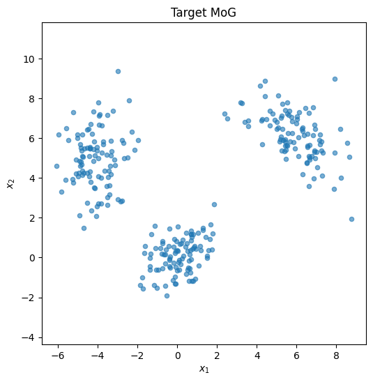
Same three-cluster MoG as the EM tutorial: 100 points each from three anisotropic Gaussians with random seed 42. To DDPM, this is just a tensor of 300 points in $\mathbb{R}^2$, it has no idea three Gaussians produced it.
```python theme={null}
import numpy as np
import torch
import torch.nn as nn
import torch.nn.functional as F
import matplotlib.pyplot as plt
# Reproducibility: identical seed across runs so this MoG matches the one
# used in the EM tutorial.
torch.manual_seed(42)
np.random.seed(42)
device = torch.device("cuda" if torch.cuda.is_available() else "cpu")
# Build the target distribution as 300 i.i.d. samples from a 3-component MoG.
# DDPM never sees the cluster labels, means, or covariances - only the
# 300x2 tensor of points. Recovering the structure from raw points alone
# is the whole point.
n_samples = 300
cluster1 = np.random.multivariate_normal([0, 0], [[1, 0.5], [0.5, 1]], n_samples // 3)
cluster2 = np.random.multivariate_normal([6, 6], [[1.5, -0.7], [-0.7, 1.5]], n_samples // 3)
cluster3 = np.random.multivariate_normal([-4, 5], [[0.8, 0], [0, 2.0]], n_samples // 3)
data_np = np.vstack([cluster1, cluster2, cluster3]).astype(np.float32)
data = torch.from_numpy(data_np).to(device)
```
In the [EM for MoG tutorial](/aiml-common/lectures/mixture-of-gaussians/em-gaussian-mixture/em-example-mog/em_example_mog) you saw the **Expectation-Maximization** algorithm *fit* a Mixture of Gaussians: given data, recover the three component means, covariances, and weights.
Here you do the opposite. You *generate* new samples from the same MoG using **Denoising Diffusion Probabilistic Models** (DDPM, Ho et al. 2020), without ever telling the model that the target distribution has three components, or what their parameters are. The model only sees data points and must learn to produce more.
The 2D MoG is the cleanest place to build intuition: every step of the forward and reverse processes can be plotted directly. The same recipe scales to images, audio, and trajectories by swapping the small MLP below for a U-Net and using more diffusion steps.
## The target distribution
Same three-cluster MoG as the EM tutorial: 100 points each from three anisotropic Gaussians with random seed 42. To DDPM, this is just a tensor of 300 points in $\mathbb{R}^2$, it has no idea three Gaussians produced it.
```python theme={null}
import numpy as np
import torch
import torch.nn as nn
import torch.nn.functional as F
import matplotlib.pyplot as plt
# Reproducibility: identical seed across runs so this MoG matches the one
# used in the EM tutorial.
torch.manual_seed(42)
np.random.seed(42)
device = torch.device("cuda" if torch.cuda.is_available() else "cpu")
# Build the target distribution as 300 i.i.d. samples from a 3-component MoG.
# DDPM never sees the cluster labels, means, or covariances - only the
# 300x2 tensor of points. Recovering the structure from raw points alone
# is the whole point.
n_samples = 300
cluster1 = np.random.multivariate_normal([0, 0], [[1, 0.5], [0.5, 1]], n_samples // 3)
cluster2 = np.random.multivariate_normal([6, 6], [[1.5, -0.7], [-0.7, 1.5]], n_samples // 3)
cluster3 = np.random.multivariate_normal([-4, 5], [[0.8, 0], [0, 2.0]], n_samples // 3)
data_np = np.vstack([cluster1, cluster2, cluster3]).astype(np.float32)
data = torch.from_numpy(data_np).to(device)
```
 ## The forward (noising) process
DDPM defines a fixed Markov chain that gradually adds Gaussian noise to a data point until, after $T$ steps, it is indistinguishable from pure noise:
$q(x_t \mid x_{t-1}) = \mathcal{N}\!\left(x_t;\; \sqrt{1-\beta_t}\, x_{t-1},\; \beta_t I\right)$
$\beta_1, \dots, \beta_T$ is the **variance schedule**. With $\alpha_t = 1 - \beta_t$ and $\bar\alpha_t = \prod_{s=1}^t \alpha_s$, the chain has a closed-form jump from any $x_0$ directly to $x_t$:
$q(x_t \mid x_0) = \mathcal{N}\!\left(x_t;\; \sqrt{\bar\alpha_t}\, x_0,\; (1-\bar\alpha_t) I\right)$
This shortcut is what makes DDPM training cheap: you never simulate the chain step by step during training, you sample $t$, jump straight to $x_t$, and learn from there.
```python theme={null}
# Forward-process hyperparameters. T is the number of noising steps;
# `betas` is the variance schedule beta_1..beta_T (small at t=0, larger at t=T-1).
# Linear schedule from 1e-4 to 0.02 is the original DDPM choice (Ho et al. 2020).
T = 500
betas = torch.linspace(1e-4, 0.02, T, device=device)
alphas = 1.0 - betas # alpha_t = 1 - beta_t
alpha_bars = torch.cumprod(alphas, dim=0) # bar_alpha_t = prod_{s=1}^t alpha_s
def q_sample(x0, t, eps=None):
"""Closed-form jump from x_0 directly to x_t.
Because every forward step is linear-Gaussian, the marginal q(x_t | x_0)
has a closed form and we never have to simulate the chain step by step:
x_t = sqrt(bar_alpha_t) * x_0 + sqrt(1 - bar_alpha_t) * eps, eps ~ N(0, I).
"""
if eps is None:
eps = torch.randn_like(x0)
# Index the schedule at each example's timestep, then unsqueeze so the
# scalar coefficient broadcasts across the 2-D point dimension.
sqrt_ab = alpha_bars[t].sqrt().unsqueeze(-1)
sqrt_omab = (1 - alpha_bars[t]).sqrt().unsqueeze(-1)
return sqrt_ab * x0 + sqrt_omab * eps
```
## The forward (noising) process
DDPM defines a fixed Markov chain that gradually adds Gaussian noise to a data point until, after $T$ steps, it is indistinguishable from pure noise:
$q(x_t \mid x_{t-1}) = \mathcal{N}\!\left(x_t;\; \sqrt{1-\beta_t}\, x_{t-1},\; \beta_t I\right)$
$\beta_1, \dots, \beta_T$ is the **variance schedule**. With $\alpha_t = 1 - \beta_t$ and $\bar\alpha_t = \prod_{s=1}^t \alpha_s$, the chain has a closed-form jump from any $x_0$ directly to $x_t$:
$q(x_t \mid x_0) = \mathcal{N}\!\left(x_t;\; \sqrt{\bar\alpha_t}\, x_0,\; (1-\bar\alpha_t) I\right)$
This shortcut is what makes DDPM training cheap: you never simulate the chain step by step during training, you sample $t$, jump straight to $x_t$, and learn from there.
```python theme={null}
# Forward-process hyperparameters. T is the number of noising steps;
# `betas` is the variance schedule beta_1..beta_T (small at t=0, larger at t=T-1).
# Linear schedule from 1e-4 to 0.02 is the original DDPM choice (Ho et al. 2020).
T = 500
betas = torch.linspace(1e-4, 0.02, T, device=device)
alphas = 1.0 - betas # alpha_t = 1 - beta_t
alpha_bars = torch.cumprod(alphas, dim=0) # bar_alpha_t = prod_{s=1}^t alpha_s
def q_sample(x0, t, eps=None):
"""Closed-form jump from x_0 directly to x_t.
Because every forward step is linear-Gaussian, the marginal q(x_t | x_0)
has a closed form and we never have to simulate the chain step by step:
x_t = sqrt(bar_alpha_t) * x_0 + sqrt(1 - bar_alpha_t) * eps, eps ~ N(0, I).
"""
if eps is None:
eps = torch.randn_like(x0)
# Index the schedule at each example's timestep, then unsqueeze so the
# scalar coefficient broadcasts across the 2-D point dimension.
sqrt_ab = alpha_bars[t].sqrt().unsqueeze(-1)
sqrt_omab = (1 - alpha_bars[t]).sqrt().unsqueeze(-1)
return sqrt_ab * x0 + sqrt_omab * eps
```
 ## The reverse (denoising) process
Generation is the forward process run backwards. We *learn* a Gaussian transition
$p_\theta(x_{t-1} \mid x_t) = \mathcal{N}\!\left(x_{t-1};\; \mu_\theta(x_t, t),\; \sigma_t^2 I\right)$
Ho et al. reparameterize the mean by training a network $\epsilon_\theta(x_t, t)$ to predict the **noise** that was added when producing $x_t$ from $x_0$. The mean is then
$\mu_\theta(x_t, t) = \frac{1}{\sqrt{\alpha_t}} \left( x_t - \frac{1-\alpha_t}{\sqrt{1-\bar\alpha_t}}\, \epsilon_\theta(x_t, t) \right)$
and the entire variational lower bound collapses to a simple denoising objective:
$L_{\text{simple}} = \mathbb{E}_{x_0, t, \epsilon}\!\left[\,\left\| \epsilon - \epsilon_\theta\!\left(\sqrt{\bar\alpha_t}\, x_0 + \sqrt{1-\bar\alpha_t}\, \epsilon,\; t\right) \right\|^2\,\right]$
No KL divergence to manage, no encoder, no posterior approximation, pure regression on noise.
### The noise predictor
For 2D data, $\epsilon_\theta$ is a small MLP. The only non-obvious piece is the **time embedding**: the network must condition on which timestep $t$ we are denoising. The conventional trick is sinusoidal positional features (same idea as transformers).
```python theme={null}
class SinusoidalTimeEmbedding(nn.Module):
"""Transformer-style positional encoding of the diffusion timestep.
A single network handles every t in {0, ..., T-1}, so it needs to know
*which* noise level it is denoising. The sin/cos embedding (used in
transformers and the original DDPM paper) gives a smooth, continuous
representation of t at many frequencies.
"""
def __init__(self, dim):
super().__init__()
self.dim = dim
def forward(self, t):
half = self.dim // 2
# Geometric series of frequencies spanning short to long timescales.
freqs = torch.exp(-np.log(10000) * torch.arange(half, device=t.device) / half)
emb = t.float().unsqueeze(-1) * freqs
return torch.cat([emb.sin(), emb.cos()], dim=-1)
class NoisePredictor(nn.Module):
"""eps_theta(x_t, t): predicts the noise that produced x_t.
The network output is NOT the reverse-step mean mu_theta; it is the
estimated 2-D noise vector eps_hat. The mean is computed analytically
from eps_hat in the sampling loop via the Ho et al. reparameterisation
(see the formula in the sampling cell). Equivalent parameterisations
exist (predict mu directly, or predict x_0), but eps-prediction is
better-conditioned because eps ~ N(0, I) at every timestep.
A small MLP suffices for 2-D data; for images this becomes a U-Net.
"""
def __init__(self, time_dim=64, hidden=128):
super().__init__()
# Project the raw sin/cos embedding through a tiny MLP (standard DDPM trick).
self.time_emb = nn.Sequential(
SinusoidalTimeEmbedding(time_dim),
nn.Linear(time_dim, time_dim), nn.SiLU(),
nn.Linear(time_dim, time_dim),
)
# Concatenate (x_t, time-embedding) -> 4-layer MLP. Output is the
# 2-D noise estimate eps_hat (same shape as x_t), NOT the reverse-step mean.
self.net = nn.Sequential(
nn.Linear(2 + time_dim, hidden), nn.SiLU(),
nn.Linear(hidden, hidden), nn.SiLU(),
nn.Linear(hidden, hidden), nn.SiLU(),
nn.Linear(hidden, 2), # eps_hat in R^2; reverse mean derived from it
)
def forward(self, x, t):
# Concatenate the noisy point with its timestep embedding.
h = torch.cat([x, self.time_emb(t)], dim=-1)
return self.net(h)
model = NoisePredictor().to(device)
```
## Training
The training loop is one of the simplest in modern generative modeling:
1. Sample a batch from $p_{\text{data}}$.
2. Sample a random timestep $t \sim \text{Uniform}(1, T)$ for each example.
3. Sample noise $\epsilon \sim \mathcal{N}(0, I)$ and form $x_t$ via the closed-form forward jump.
4. Predict $\hat\epsilon = \epsilon_\theta(x_t, t)$.
5. Minimize $\|\epsilon - \hat\epsilon\|^2$.
That is the whole algorithm.
```python theme={null}
optim = torch.optim.Adam(model.parameters(), lr=1e-3)
batch_size = 256
n_steps = 4000
losses = []
# DDPM training is stochastic over (x_0, t, eps) triples.
# At each step we sample a clean point, a random diffusion timestep, and a
# noise vector, then ask the network to recover that noise.
for step in range(n_steps):
# 1. Random minibatch of clean data points (with replacement; tiny dataset).
idx = torch.randint(0, data.shape[0], (batch_size,), device=device)
x0 = data[idx]
# 2. Independent random timestep per example. Mixing all noise levels
# in one batch is what teaches the network ALL t in one model.
t = torch.randint(0, T, (batch_size,), device=device)
# 3. Form x_t = sqrt(bar_alpha_t) x_0 + sqrt(1 - bar_alpha_t) eps in closed form.
eps = torch.randn_like(x0)
xt = q_sample(x0, t, eps)
# 4. Predict the noise and minimise MSE against the true eps.
# This is L_simple from Ho et al.: a reweighted ELBO that works
# dramatically better in practice than the raw variational bound.
eps_hat = model(xt, t)
loss = F.mse_loss(eps_hat, eps)
optim.zero_grad()
loss.backward()
optim.step()
losses.append(loss.item())
if (step + 1) % 1000 == 0:
print(f"step {step + 1:>5d} loss {float(np.mean(losses[-500:])):.4f}")
```
```output theme={null}
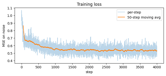
step 1000 loss 0.5713
```
```output theme={null}
step 2000 loss 0.5401
```
```output theme={null}
step 3000 loss 0.5375
```
```output theme={null}
step 4000 loss 0.5341
```
## The reverse (denoising) process
Generation is the forward process run backwards. We *learn* a Gaussian transition
$p_\theta(x_{t-1} \mid x_t) = \mathcal{N}\!\left(x_{t-1};\; \mu_\theta(x_t, t),\; \sigma_t^2 I\right)$
Ho et al. reparameterize the mean by training a network $\epsilon_\theta(x_t, t)$ to predict the **noise** that was added when producing $x_t$ from $x_0$. The mean is then
$\mu_\theta(x_t, t) = \frac{1}{\sqrt{\alpha_t}} \left( x_t - \frac{1-\alpha_t}{\sqrt{1-\bar\alpha_t}}\, \epsilon_\theta(x_t, t) \right)$
and the entire variational lower bound collapses to a simple denoising objective:
$L_{\text{simple}} = \mathbb{E}_{x_0, t, \epsilon}\!\left[\,\left\| \epsilon - \epsilon_\theta\!\left(\sqrt{\bar\alpha_t}\, x_0 + \sqrt{1-\bar\alpha_t}\, \epsilon,\; t\right) \right\|^2\,\right]$
No KL divergence to manage, no encoder, no posterior approximation, pure regression on noise.
### The noise predictor
For 2D data, $\epsilon_\theta$ is a small MLP. The only non-obvious piece is the **time embedding**: the network must condition on which timestep $t$ we are denoising. The conventional trick is sinusoidal positional features (same idea as transformers).
```python theme={null}
class SinusoidalTimeEmbedding(nn.Module):
"""Transformer-style positional encoding of the diffusion timestep.
A single network handles every t in {0, ..., T-1}, so it needs to know
*which* noise level it is denoising. The sin/cos embedding (used in
transformers and the original DDPM paper) gives a smooth, continuous
representation of t at many frequencies.
"""
def __init__(self, dim):
super().__init__()
self.dim = dim
def forward(self, t):
half = self.dim // 2
# Geometric series of frequencies spanning short to long timescales.
freqs = torch.exp(-np.log(10000) * torch.arange(half, device=t.device) / half)
emb = t.float().unsqueeze(-1) * freqs
return torch.cat([emb.sin(), emb.cos()], dim=-1)
class NoisePredictor(nn.Module):
"""eps_theta(x_t, t): predicts the noise that produced x_t.
The network output is NOT the reverse-step mean mu_theta; it is the
estimated 2-D noise vector eps_hat. The mean is computed analytically
from eps_hat in the sampling loop via the Ho et al. reparameterisation
(see the formula in the sampling cell). Equivalent parameterisations
exist (predict mu directly, or predict x_0), but eps-prediction is
better-conditioned because eps ~ N(0, I) at every timestep.
A small MLP suffices for 2-D data; for images this becomes a U-Net.
"""
def __init__(self, time_dim=64, hidden=128):
super().__init__()
# Project the raw sin/cos embedding through a tiny MLP (standard DDPM trick).
self.time_emb = nn.Sequential(
SinusoidalTimeEmbedding(time_dim),
nn.Linear(time_dim, time_dim), nn.SiLU(),
nn.Linear(time_dim, time_dim),
)
# Concatenate (x_t, time-embedding) -> 4-layer MLP. Output is the
# 2-D noise estimate eps_hat (same shape as x_t), NOT the reverse-step mean.
self.net = nn.Sequential(
nn.Linear(2 + time_dim, hidden), nn.SiLU(),
nn.Linear(hidden, hidden), nn.SiLU(),
nn.Linear(hidden, hidden), nn.SiLU(),
nn.Linear(hidden, 2), # eps_hat in R^2; reverse mean derived from it
)
def forward(self, x, t):
# Concatenate the noisy point with its timestep embedding.
h = torch.cat([x, self.time_emb(t)], dim=-1)
return self.net(h)
model = NoisePredictor().to(device)
```
## Training
The training loop is one of the simplest in modern generative modeling:
1. Sample a batch from $p_{\text{data}}$.
2. Sample a random timestep $t \sim \text{Uniform}(1, T)$ for each example.
3. Sample noise $\epsilon \sim \mathcal{N}(0, I)$ and form $x_t$ via the closed-form forward jump.
4. Predict $\hat\epsilon = \epsilon_\theta(x_t, t)$.
5. Minimize $\|\epsilon - \hat\epsilon\|^2$.
That is the whole algorithm.
```python theme={null}
optim = torch.optim.Adam(model.parameters(), lr=1e-3)
batch_size = 256
n_steps = 4000
losses = []
# DDPM training is stochastic over (x_0, t, eps) triples.
# At each step we sample a clean point, a random diffusion timestep, and a
# noise vector, then ask the network to recover that noise.
for step in range(n_steps):
# 1. Random minibatch of clean data points (with replacement; tiny dataset).
idx = torch.randint(0, data.shape[0], (batch_size,), device=device)
x0 = data[idx]
# 2. Independent random timestep per example. Mixing all noise levels
# in one batch is what teaches the network ALL t in one model.
t = torch.randint(0, T, (batch_size,), device=device)
# 3. Form x_t = sqrt(bar_alpha_t) x_0 + sqrt(1 - bar_alpha_t) eps in closed form.
eps = torch.randn_like(x0)
xt = q_sample(x0, t, eps)
# 4. Predict the noise and minimise MSE against the true eps.
# This is L_simple from Ho et al.: a reweighted ELBO that works
# dramatically better in practice than the raw variational bound.
eps_hat = model(xt, t)
loss = F.mse_loss(eps_hat, eps)
optim.zero_grad()
loss.backward()
optim.step()
losses.append(loss.item())
if (step + 1) % 1000 == 0:
print(f"step {step + 1:>5d} loss {float(np.mean(losses[-500:])):.4f}")
```
```output theme={null}
step 1000 loss 0.5713
```
```output theme={null}
step 2000 loss 0.5401
```
```output theme={null}
step 3000 loss 0.5375
```
```output theme={null}
step 4000 loss 0.5341
```
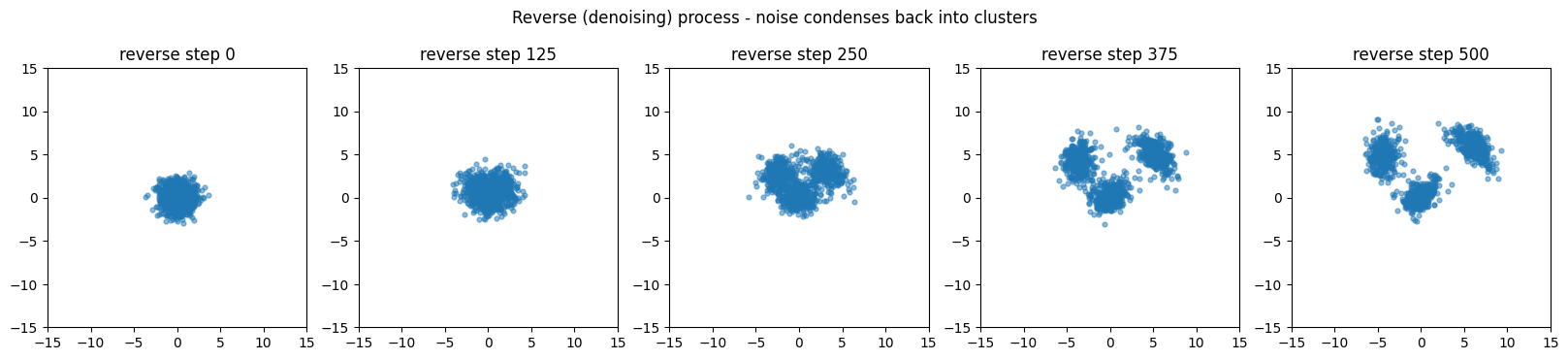
 ## Sampling: the reverse process in action
Now run the chain backwards. Start with $x_T \sim \mathcal{N}(0, I)$ and, for $t = T, T-1, \dots, 1$, take a step:
$x_{t-1} = \frac{1}{\sqrt{\alpha_t}}\!\left( x_t - \frac{1-\alpha_t}{\sqrt{1-\bar\alpha_t}}\, \epsilon_\theta(x_t, t)\right) + \sigma_t z$
with $z \sim \mathcal{N}(0, I)$ for $t > 1$ and $z = 0$ at the final step. The standard variance choice is $\sigma_t = \sqrt{\beta_t}$.
```python theme={null}
@torch.no_grad()
def sample(n=1000):
"""Run the reverse chain from pure noise back to data.
Start at x_T ~ N(0, I) and iteratively denoise down to x_0 by applying
the learned reverse transition p_theta(x_{t-1} | x_t).
"""
# 1. Initialise n samples as pure standard Gaussian noise. This is x_T.
x = torch.randn(n, 2, device=device)
trajectory = [x.cpu().numpy().copy()]
# 2. Loop t = T-1, T-2, ..., 0 (reversed range produces this order).
for t_step in reversed(range(T)):
t = torch.full((n,), t_step, device=device, dtype=torch.long)
# Predicted noise at the current step.
eps = model(x, t)
beta_t = betas[t_step]
alpha_t = alphas[t_step]
ab_t = alpha_bars[t_step]
# 3. Reverse-transition mean under the Ho et al. parameterisation:
# mu_theta(x_t, t) = (1/sqrt(alpha_t)) * (x_t - (1-alpha_t)/sqrt(1-bar_alpha_t) * eps_theta).
coef = (1 - alpha_t) / (1 - ab_t).sqrt()
mean = (x - coef * eps) / alpha_t.sqrt()
# 4. Add Langevin noise scaled by sqrt(beta_t), except at the final
# step where we want a deterministic x_0 rather than a noisy draw.
if t_step > 0:
x = mean + beta_t.sqrt() * torch.randn_like(x)
else:
x = mean
trajectory.append(x.cpu().numpy().copy())
return x.cpu().numpy(), trajectory
generated, traj = sample(n=1000)
```
## Sampling: the reverse process in action
Now run the chain backwards. Start with $x_T \sim \mathcal{N}(0, I)$ and, for $t = T, T-1, \dots, 1$, take a step:
$x_{t-1} = \frac{1}{\sqrt{\alpha_t}}\!\left( x_t - \frac{1-\alpha_t}{\sqrt{1-\bar\alpha_t}}\, \epsilon_\theta(x_t, t)\right) + \sigma_t z$
with $z \sim \mathcal{N}(0, I)$ for $t > 1$ and $z = 0$ at the final step. The standard variance choice is $\sigma_t = \sqrt{\beta_t}$.
```python theme={null}
@torch.no_grad()
def sample(n=1000):
"""Run the reverse chain from pure noise back to data.
Start at x_T ~ N(0, I) and iteratively denoise down to x_0 by applying
the learned reverse transition p_theta(x_{t-1} | x_t).
"""
# 1. Initialise n samples as pure standard Gaussian noise. This is x_T.
x = torch.randn(n, 2, device=device)
trajectory = [x.cpu().numpy().copy()]
# 2. Loop t = T-1, T-2, ..., 0 (reversed range produces this order).
for t_step in reversed(range(T)):
t = torch.full((n,), t_step, device=device, dtype=torch.long)
# Predicted noise at the current step.
eps = model(x, t)
beta_t = betas[t_step]
alpha_t = alphas[t_step]
ab_t = alpha_bars[t_step]
# 3. Reverse-transition mean under the Ho et al. parameterisation:
# mu_theta(x_t, t) = (1/sqrt(alpha_t)) * (x_t - (1-alpha_t)/sqrt(1-bar_alpha_t) * eps_theta).
coef = (1 - alpha_t) / (1 - ab_t).sqrt()
mean = (x - coef * eps) / alpha_t.sqrt()
# 4. Add Langevin noise scaled by sqrt(beta_t), except at the final
# step where we want a deterministic x_0 rather than a noisy draw.
if t_step > 0:
x = mean + beta_t.sqrt() * torch.randn_like(x)
else:
x = mean
trajectory.append(x.cpu().numpy().copy())
return x.cpu().numpy(), trajectory
generated, traj = sample(n=1000)
```
 ## Did it work?
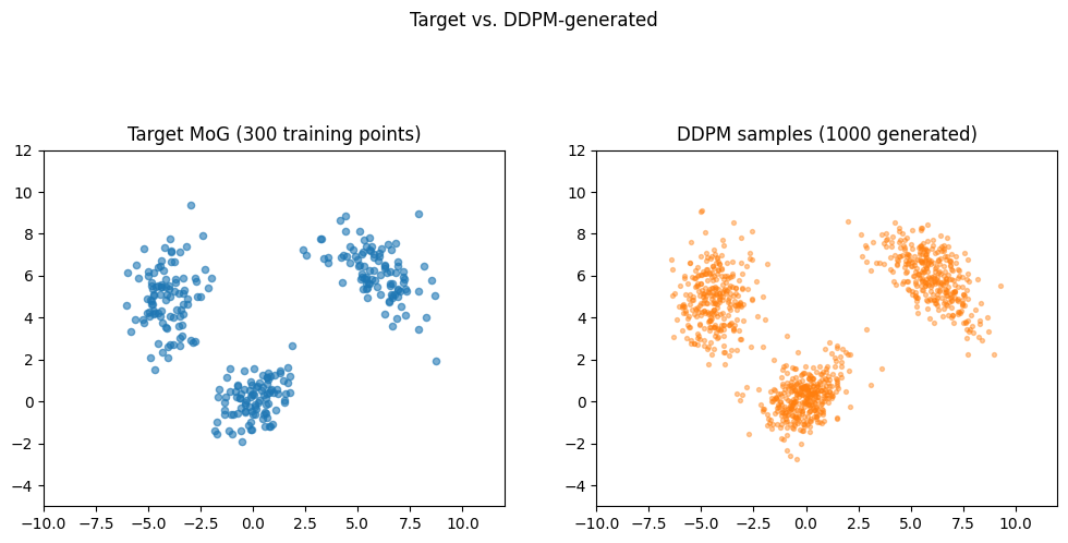
Compare the generated samples to the original training data. The model never learned that there are three components, that they are Gaussian, or where their centers are, it only saw 300 data points and a noise-prediction objective. If the three clusters reappear in the generated cloud, the diffusion model has captured the data distribution.
## Did it work?
Compare the generated samples to the original training data. The model never learned that there are three components, that they are Gaussian, or where their centers are, it only saw 300 data points and a noise-prediction objective. If the three clusters reappear in the generated cloud, the diffusion model has captured the data distribution.
 ## Connections to other concepts
* **Black-box density modeling.** DDPM treats $p_{\text{data}}$ as opaque. Compare with EM, which assumes a parametric mixture form and fits its parameters.
* **Same recipe, bigger backbone.** Replace the 4-layer MLP with a U-Net and the same noise-prediction objective generates 256×256 images. The schedule, the closed-form forward jump, and the training loop do not change.
* **Conditional and guided generation.** Condition $\epsilon_\theta(x_t, t, y)$ on a label, prompt, or class to obtain conditional models, and combine with classifier-free guidance to trade diversity for fidelity.
* **Latent diffusion.** Run the entire chain inside a learned latent space (encode → diffuse in latents → decode) for orders-of-magnitude faster image generation.
* **Score-based unification.** The [Score MoG Tutorial](/aiml-common/lectures/diffusion/score-based/score-mog-example/score_mog_example) trains $s_\theta(x, \sigma)$ directly, a network that approximates $\nabla \log p_\sigma(x)$. DDPM's noise predictor $\epsilon_\theta(x_t, t)$ is, up to a known scaling, a score predictor at the variance-preserving SDE. Same network, different parameterization.
* **Faster, deterministic sampling.** The [DDIM tutorial](/aiml-common/lectures/diffusion/ddim/ddim_mog_tutorial) reuses this same trained model with a different sampler that takes a fraction of the steps and is deterministic, opening the door to latent interpolation and editing.
## References
1. Ho, Jain, Abbeel. *Denoising Diffusion Probabilistic Models.* NeurIPS 2020. [arxiv.org/abs/2006.11239](https://arxiv.org/abs/2006.11239)
2. Sohl-Dickstein et al. *Deep Unsupervised Learning using Nonequilibrium Thermodynamics.* ICML 2015. [arxiv.org/abs/1503.03585](https://arxiv.org/abs/1503.03585)
3. Nichol, Dhariwal. *Improved Denoising Diffusion Probabilistic Models.* ICML 2021. [arxiv.org/abs/2102.09672](https://arxiv.org/abs/2102.09672)
## PyTorch reference
| PyTorch class | Description |
| ---------------------------------------------------------------------------------------- | ----------------------------------------------------------------------------- |
| [`nn.Sequential`](https://docs.pytorch.org/docs/2.12/generated/torch.nn.Sequential.html) | A sequential container. |
| [`nn.Linear`](https://docs.pytorch.org/docs/2.12/generated/torch.nn.Linear.html) | Applies an affine linear transformation to the incoming data: $y = xA^T + b$. |
| [`nn.SiLU`](https://docs.pytorch.org/docs/2.12/generated/torch.nn.SiLU.html) | Applies the Sigmoid Linear Unit (SiLU) function, element-wise. |
***
[Edit this page on GitHub](https://github.com/aegean-ai/eaia/edit/main/src/aiml-common/lectures/diffusion/ddpm/ddpm_mog_tutorial.mdx) or [file an issue](https://github.com/aegean-ai/eaia/issues/new/choose).
## Connections to other concepts
* **Black-box density modeling.** DDPM treats $p_{\text{data}}$ as opaque. Compare with EM, which assumes a parametric mixture form and fits its parameters.
* **Same recipe, bigger backbone.** Replace the 4-layer MLP with a U-Net and the same noise-prediction objective generates 256×256 images. The schedule, the closed-form forward jump, and the training loop do not change.
* **Conditional and guided generation.** Condition $\epsilon_\theta(x_t, t, y)$ on a label, prompt, or class to obtain conditional models, and combine with classifier-free guidance to trade diversity for fidelity.
* **Latent diffusion.** Run the entire chain inside a learned latent space (encode → diffuse in latents → decode) for orders-of-magnitude faster image generation.
* **Score-based unification.** The [Score MoG Tutorial](/aiml-common/lectures/diffusion/score-based/score-mog-example/score_mog_example) trains $s_\theta(x, \sigma)$ directly, a network that approximates $\nabla \log p_\sigma(x)$. DDPM's noise predictor $\epsilon_\theta(x_t, t)$ is, up to a known scaling, a score predictor at the variance-preserving SDE. Same network, different parameterization.
* **Faster, deterministic sampling.** The [DDIM tutorial](/aiml-common/lectures/diffusion/ddim/ddim_mog_tutorial) reuses this same trained model with a different sampler that takes a fraction of the steps and is deterministic, opening the door to latent interpolation and editing.
## References
1. Ho, Jain, Abbeel. *Denoising Diffusion Probabilistic Models.* NeurIPS 2020. [arxiv.org/abs/2006.11239](https://arxiv.org/abs/2006.11239)
2. Sohl-Dickstein et al. *Deep Unsupervised Learning using Nonequilibrium Thermodynamics.* ICML 2015. [arxiv.org/abs/1503.03585](https://arxiv.org/abs/1503.03585)
3. Nichol, Dhariwal. *Improved Denoising Diffusion Probabilistic Models.* ICML 2021. [arxiv.org/abs/2102.09672](https://arxiv.org/abs/2102.09672)
## PyTorch reference
| PyTorch class | Description |
| ---------------------------------------------------------------------------------------- | ----------------------------------------------------------------------------- |
| [`nn.Sequential`](https://docs.pytorch.org/docs/2.12/generated/torch.nn.Sequential.html) | A sequential container. |
| [`nn.Linear`](https://docs.pytorch.org/docs/2.12/generated/torch.nn.Linear.html) | Applies an affine linear transformation to the incoming data: $y = xA^T + b$. |
| [`nn.SiLU`](https://docs.pytorch.org/docs/2.12/generated/torch.nn.SiLU.html) | Applies the Sigmoid Linear Unit (SiLU) function, element-wise. |
***
[Edit this page on GitHub](https://github.com/aegean-ai/eaia/edit/main/src/aiml-common/lectures/diffusion/ddpm/ddpm_mog_tutorial.mdx) or [file an issue](https://github.com/aegean-ai/eaia/issues/new/choose).