> ## Documentation Index
> Fetch the complete documentation index at: https://aegean.ai/llms.txt
> Use this file to discover all available pages before exploring further.
# Score-based generative models
> A guided walkthrough of Yang Song's MIT CBMM tutorial — the score function, score matching, the forward and reverse SDE, and the probability-flow ODE that connect DDPM, DDIM, and modern diffusion samplers.
The score-based view treats generative modeling as **estimating the gradient of the log-density**, $\nabla_x \log p_t(x)$, rather than the density itself. The DDPM training objective and DDIM sampler you have already seen are special cases: DDPM trains a noise predictor $\epsilon_\theta(x_t, t)$ which is, up to a known scaling factor, an estimate of the score; DDIM's deterministic limit is the *probability-flow ODE* derived from the score-SDE.
This page is a tutorial reading guide for Yang Song's MIT CBMM lecture below. Each section opens with one slide from the *Topography of the Noise* deck and walks through the corresponding lecture segment. You can read straight through, or skip into the video at the timestamp noted in each section.
## The intractable wall
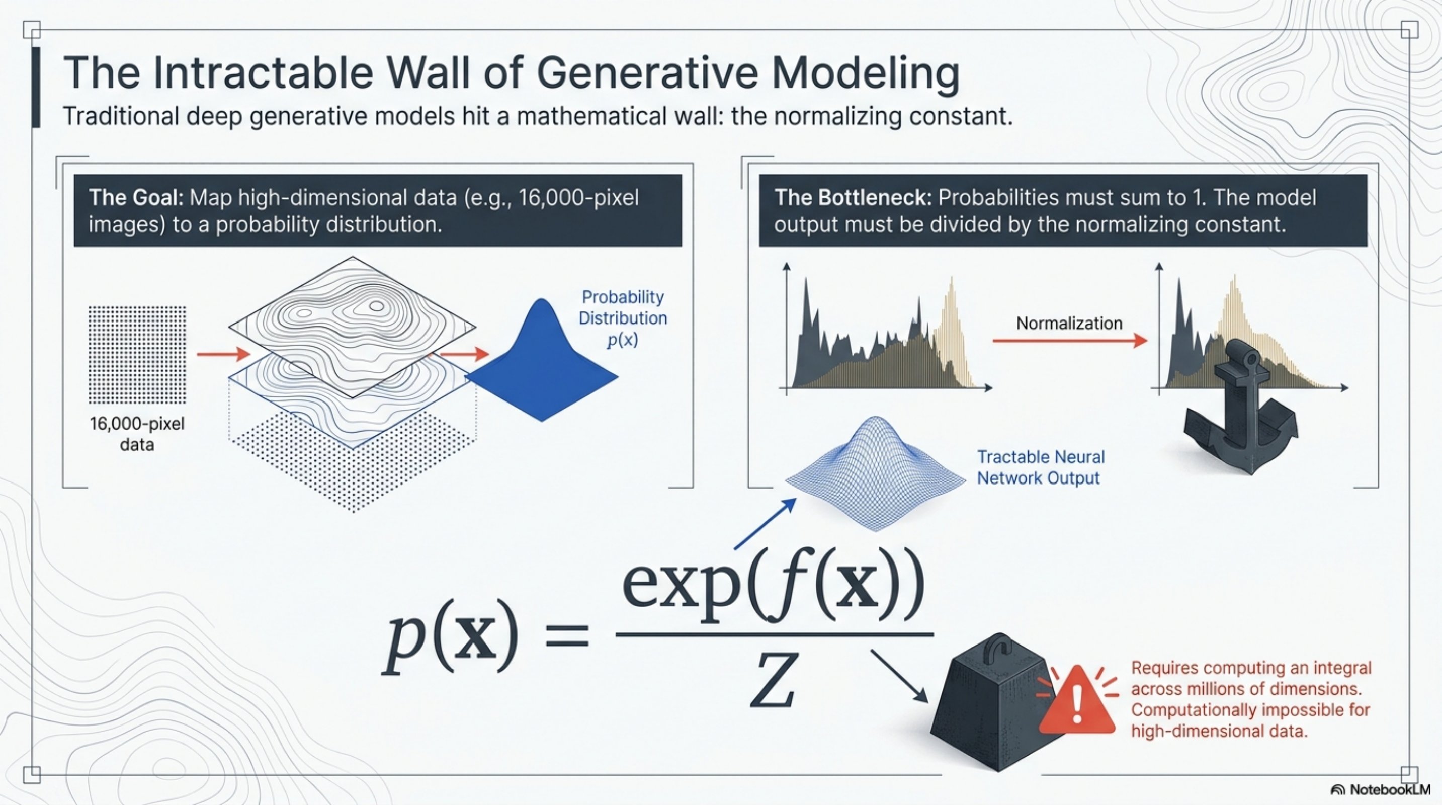
A neural network is a black box from $x \in \mathbb{R}^D$ to a scalar $f_\theta(x) \in \mathbb{R}$. To turn that scalar into a probability density you need
$$
p_\theta(x) \;=\; \frac{\exp(f_\theta(x))}{Z_\theta}, \qquad Z_\theta = \int \exp(f_\theta(x))\, dx.
$$
For images, $D$ is in the tens of thousands. The integral $Z_\theta$ has no closed form and Monte-Carlo estimates are useless at this dimensionality. Every classical likelihood-based generative model — autoregressive, normalizing flows, VAEs — makes some architectural sacrifice to keep $Z_\theta$ tractable: factorize over coordinates, restrict to invertible maps, or optimize a lower bound. Each restriction either limits expressiveness or limits how directly you can score real samples.
The score-based view simply refuses to compute $Z_\theta$.
**Lecture:** open at [≈ 8:00](https://www.youtube.com/watch?v=wMmqCMwuM2Q\&t=480s) for Yang Song's framing of this bottleneck.
## Trade the map for a compass: the score function
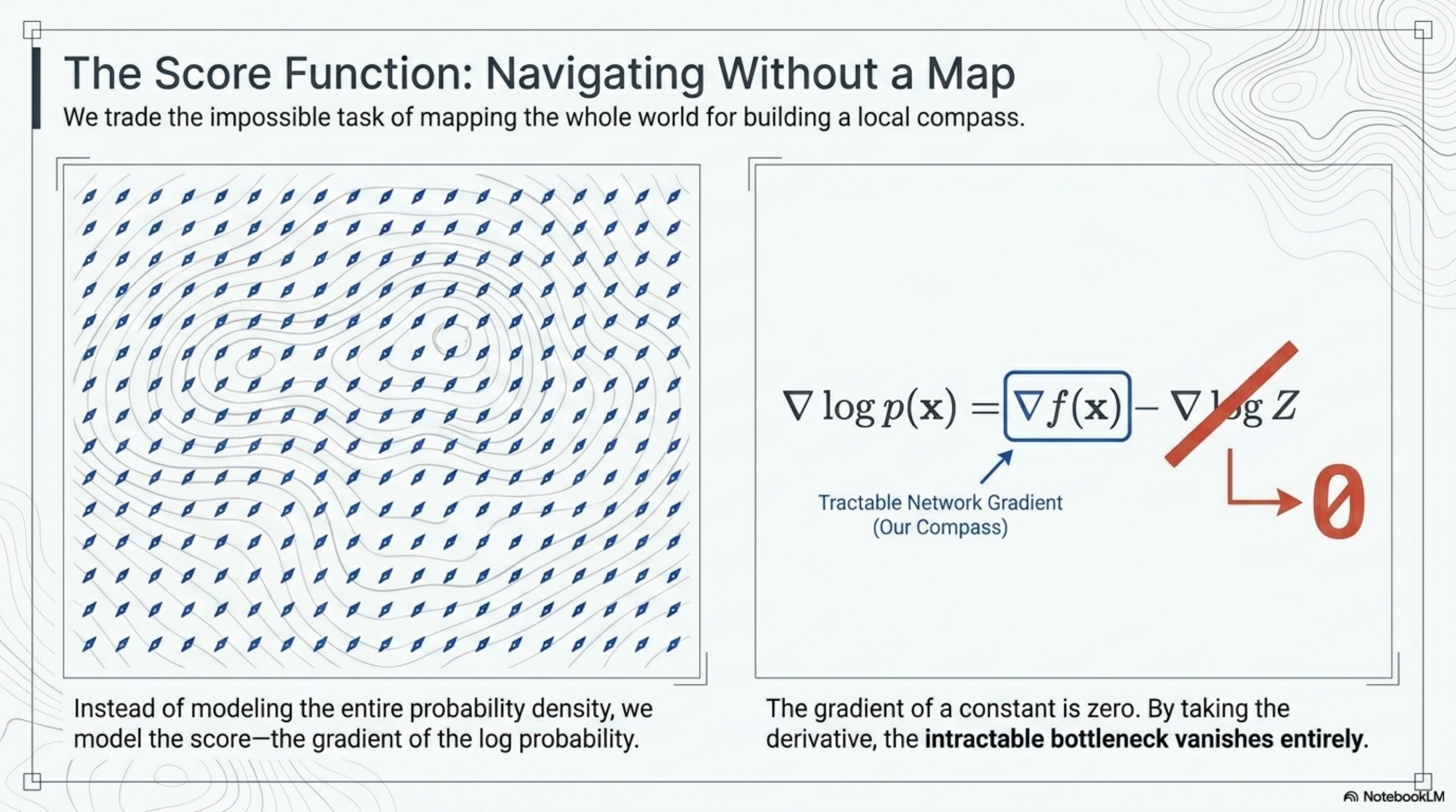
Take the gradient of the log of both sides:
$$
s_\theta(x) \;:=\; \nabla_x \log p_\theta(x) \;=\; \nabla_x f_\theta(x) - \cancel{\nabla_x \log Z_\theta} \;=\; \nabla_x f_\theta(x).
$$
The gradient of a constant is zero. The intractable $Z_\theta$ vanishes from the gradient field, and what remains — the **score** — is something a neural network can output directly: a vector field with the same shape as the input.
A density $p(x)$ is a *map* of where probability mass lives. The score $\nabla_x \log p(x)$ is a *compass* that tells you, at any $x$, which direction increases log-density. You don't need the map to navigate: a compass at every point is enough to roll downhill toward the data.
**Lecture:** [≈ 18:00](https://www.youtube.com/watch?v=wMmqCMwuM2Q\&t=1080s).
## The low-density trap
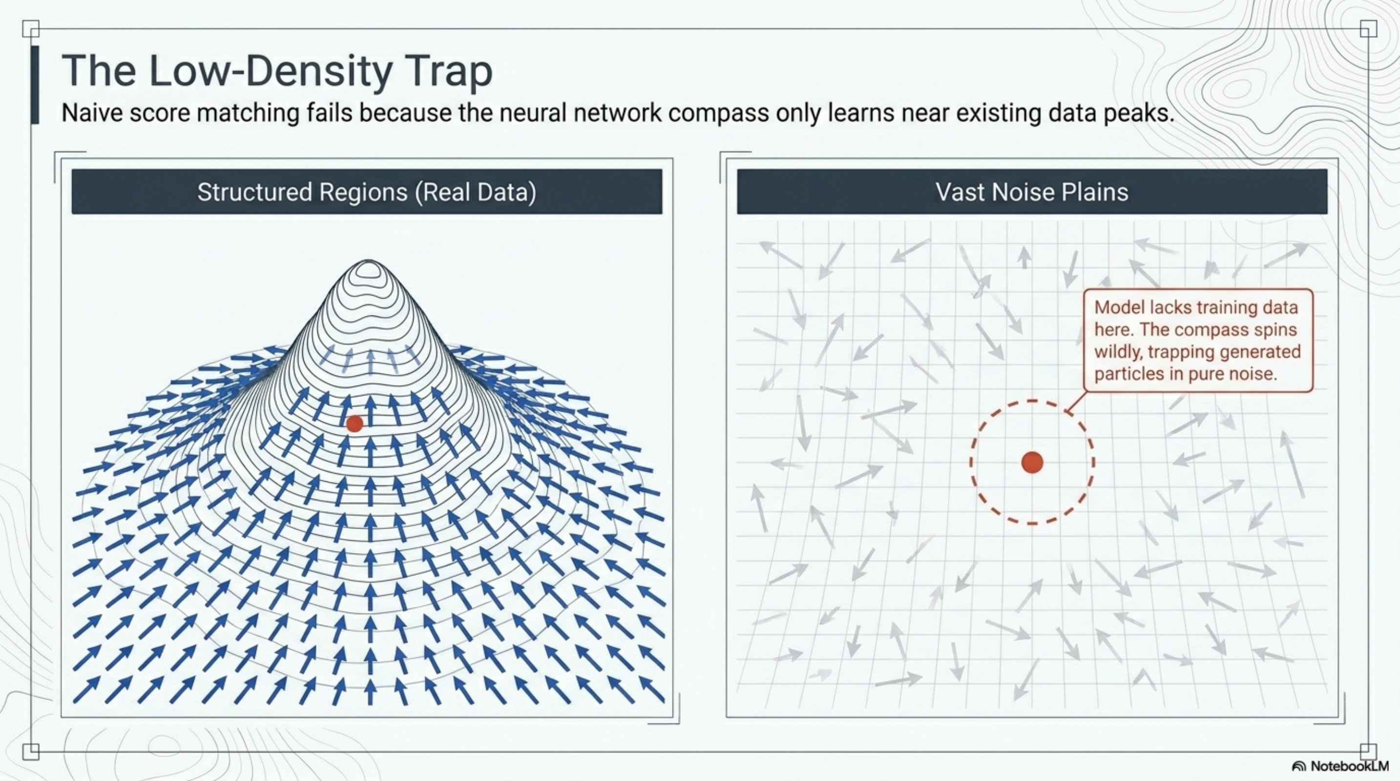
Naive score matching has a fatal flaw. Training data $\{x_i\} \sim p_{\text{data}}$ lives on (or near) a thin manifold inside an enormous ambient space. Score matching minimizes the expected squared error between $s_\theta(x)$ and the true score, with the expectation taken **under $p_{\text{data}}$**:
$$
\mathcal{L}(\theta) \;=\; \mathbb{E}_{x \sim p_{\text{data}}}\!\left[\,\bigl\|\, s_\theta(x) - \nabla_x \log p_{\text{data}}(x) \,\bigr\|^2\right].
$$
The model is only trained where the data lives. Far from the manifold the loss puts no weight at all, so the learned compass spins randomly there. At sampling time you start from a Gaussian sample — pure noise, with overwhelming probability *far* from the data — and the compass gives you no signal to follow back. You stay lost.
This is *the* problem the rest of the lecture is built to solve.
**Lecture:** [≈ 36:00](https://www.youtube.com/watch?v=wMmqCMwuM2Q\&t=2160s).
## Noise as a bridge
The fix is physical. Inject Gaussian noise into the data and let it spread the probability mass outward over time. Sharp spikes broaden into smooth bumps, empty valleys fill in. After enough noise, the landscape has a non-zero, smoothly-varying gradient *everywhere* — and a network trained to match the score of the noisy distribution will have a well-defined target across the whole space.
This is the non-equilibrium thermodynamics picture: a drop of dye in water starts as a localized concentration ($t=0$) and ends as a uniform mixture ($t \to \infty$). Score-based models reverse that diffusion. The forward process buys you a usable signal across the noise plain; the reverse process trades it back for samples on the data manifold.
This is exactly the [forward noising process](/aiml-common/lectures/diffusion/brownian-motion/brownian_motion) you saw in the Brownian-motion section — eight trajectories spreading from the origin — restated in the language of densities rather than particles.
**Lecture:** [≈ 38:00](https://www.youtube.com/watch?v=wMmqCMwuM2Q\&t=2280s).
## The forward SDE
In continuous time the noising process is a stochastic differential equation:
$$
dx \;=\; f(x, t)\, dt \;+\; g(t)\, dW_t, \qquad t \in [0, T],
$$
with $x_0 \sim p_{\text{data}}$ and $W_t$ a standard Wiener process.
* **Drift** $f(x, t)$: a deterministic pull. In Variance-Preserving (VP) SDEs the drift contracts $x$ toward the origin to stop variance from blowing up; in Variance-Exploding (VE) SDEs it is zero.
* **Diffusion** $g(t)$: a scalar volatility schedule controlling how fast Gaussian noise is injected.
DDPM is the **discrete-time Variance-Preserving** instance of this SDE, with the noise schedule $\beta_t$ playing the role of $f$ and $g$. The forward trajectory you trained against in the [DDPM tutorial](/aiml-common/lectures/diffusion/ddpm/ddpm_mog_tutorial) is one Euler-Maruyama discretization of exactly this SDE.
**Lecture:** [≈ 1:00:00](https://www.youtube.com/watch?v=wMmqCMwuM2Q\&t=3600s).
## Training the score network
The implicit score-matching loss
$$
\mathbb{E}_{p_{\text{data}}}\!\left[\,\tfrac{1}{2}\|s_\theta(x)\|^2 \;+\; \mathrm{tr}\!\left(\nabla_x s_\theta(x)\right)\right]
$$
removes the unknown $\nabla \log p_{\text{data}}$ via integration by parts, but the Jacobian trace requires $D$ separate backward passes — fatal for images. Three workarounds:
| Variant | Trick | Cost | Trade-off |
| ------------------- | ------------------------------------------------------------------------------------------------------------------------------------------------ | ---------------------------------- | ------------------------------------------------------------- |
| **Vanilla** | Compute $\mathrm{tr}(\nabla s_\theta)$ exactly | $O(D)$ backprops | Exact, unusable above \~1k dims |
| **Sliced** | Random unit vectors $v$; replace trace by $v^\top (\nabla s_\theta)\, v$ | $O(1)$ via Jacobian-vector product | Unbiased, higher variance |
| **Denoising (DSM)** | Perturb $x$ with kernel $q_\sigma(\tilde x \mid x)$; train against the *known* analytic score $\nabla_{\tilde x} \log q_\sigma(\tilde x \mid x)$ | $O(1)$, no Jacobians | Estimates the score of the *noisy* density, not the clean one |
DSM is the standard choice. With Gaussian perturbation $\tilde x = x + \sigma \epsilon, \epsilon \sim \mathcal{N}(0, I)$:
$$
\nabla_{\tilde x} \log q_\sigma(\tilde x \mid x) \;=\; -\frac{\tilde x - x}{\sigma^2} \;=\; -\frac{\epsilon}{\sigma},
$$
so the DSM loss reduces to a re-weighted noise-prediction loss — *this is exactly the DDPM training objective up to a $\sigma$-dependent constant*. The DDPM noise predictor $\epsilon_\theta$ and the score network $s_\theta$ are the same model with a different sign and scale.
**Lecture:** [≈ 22:00–34:00](https://www.youtube.com/watch?v=wMmqCMwuM2Q\&t=1320s) walks through all three variants.
## Reversing the SDE
Anderson's 1982 reversal theorem is the engine of generation. Every forward diffusion has a reverse-time partner:
$$
dx \;=\; \bigl[\,f(x, t) \;-\; g(t)^2\, \nabla_x \log p_t(x)\,\bigr]\, dt \;+\; g(t)\, d\bar W_t,
$$
where $d\bar W_t$ is a Wiener process running *backward* in time and $p_t$ is the marginal density at time $t$ under the forward SDE.
The only unknown on the right-hand side is $\nabla_x \log p_t(x)$ — and that is precisely what the score network was trained to estimate. Substitute $s_\theta(x, t) \approx \nabla_x \log p_t(x)$ and you have a generator: start from a sample of $p_T \approx \mathcal{N}(0, \sigma_T^2 I)$ and integrate backward to $t = 0$ to land on the data manifold.
This is the same idea as **annealed Langevin dynamics**: at each $t$, take a step downhill along $s_\theta(\cdot, t)$ plus a noise kick, and gradually decrease the noise level. The continuous-time SDE view subsumes the discrete annealed-Langevin sampler used in NCSN and the ancestral sampler used in DDPM.
**Lecture:** [≈ 1:04:00](https://www.youtube.com/watch?v=wMmqCMwuM2Q\&t=3840s).
## Two solvers: stochastic vs deterministic
For every score-SDE there is a deterministic ODE that produces *the same marginal densities* $p_t$:
$$
\frac{dx}{dt} \;=\; f(x, t) \;-\; \tfrac{1}{2}\, g(t)^2\, \nabla_x \log p_t(x).
$$
This is the **probability-flow ODE**. The diffusion term is gone — only drift remains — but the family of distributions $\{p_t\}$ swept out by the ODE is identical to the SDE's. Two consequences:
1. **Fewer steps.** ODE solvers (Heun, DPM-Solver, RK45) converge in 20–50 NFEs versus the 500–1000 needed by reverse-SDE samplers. This is what production systems use.
2. **A bijection between data and noise.** The ODE is invertible. Each data point maps to a unique latent code in the prior, which gives you exact log-likelihoods (via the change-of-variables formula and Hutchinson's estimator) and a meaningful semantic latent space — for free, after training.
The deterministic DDIM sampler ($\eta = 0$) you implemented in the [DDIM tutorial](/aiml-common/lectures/diffusion/ddim/ddim_mog_tutorial) is a first-order discretization of this ODE.
**Lecture:** [≈ 1:07:00](https://www.youtube.com/watch?v=wMmqCMwuM2Q\&t=4020s).
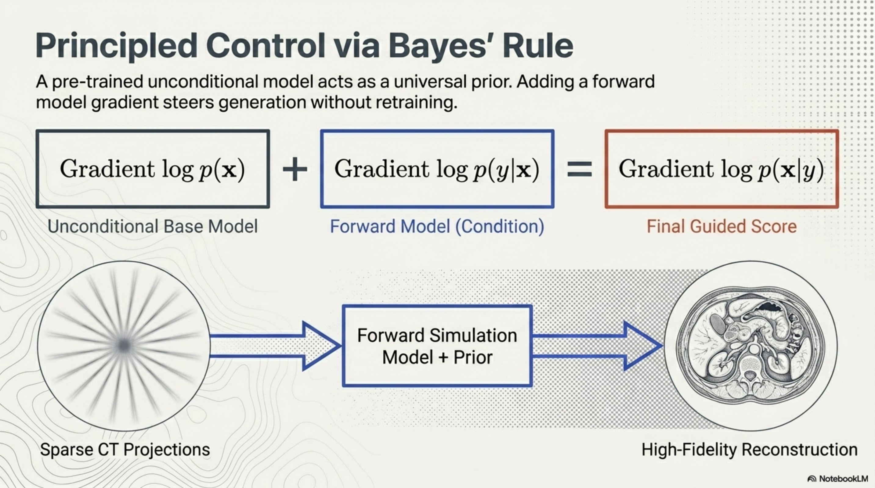
## Conditional generation via Bayes' rule
Conditioning is almost free in score space. Take logs and gradients of Bayes' rule:
$$
\nabla_x \log p(x \mid y) \;=\; \underbrace{\nabla_x \log p(x)}_{\text{unconditional score}} \;+\; \underbrace{\nabla_x \log p(y \mid x)}_{\text{condition / likelihood}}.
$$
The unconditional score is your already-trained diffusion prior. The likelihood term comes from a forward model — a classifier, a degradation operator, a physics simulator. Add the two scores at every step of the reverse SDE/ODE and you sample from the posterior $p(x \mid y)$ without retraining the prior.
This single identity unifies a remarkable range of applications:
* **Inverse problems in medical imaging.** $y$ is a sparse-view CT sinogram; $p(y \mid x)$ is the (linear, known) Radon transform plus measurement noise. The diffusion prior is a generic image model trained once, and the same prior reconstructs MRI, CT, and microscopy images.
* **Class-conditional generation.** $p(y \mid x)$ is a classifier; classifier guidance (and its classifier-free cousin) is the same idea.
* **Text-to-image.** $y$ is a text embedding; the conditional score is approximated jointly with the unconditional one in a single network.
**Lecture:** [≈ 1:14:00](https://www.youtube.com/watch?v=wMmqCMwuM2Q\&t=4440s).
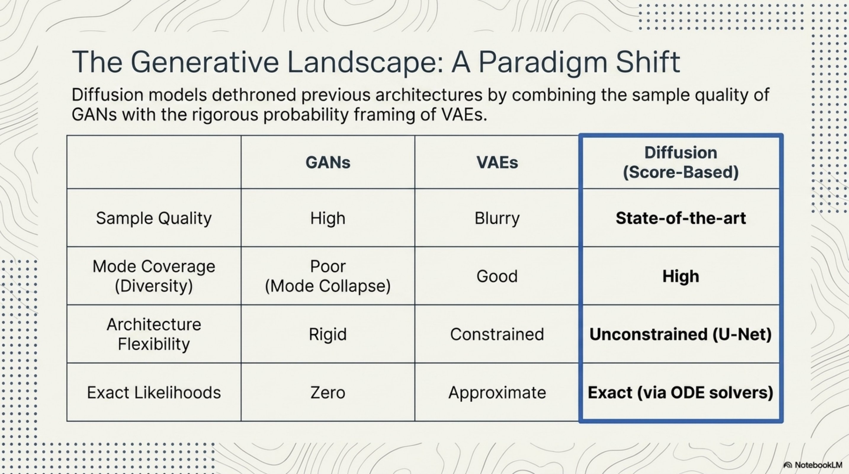
## Where score-based models fit
The score-SDE framework inherits the strengths of earlier families and shares few of their weaknesses:
* **Sample quality** rivals or exceeds GANs on benchmark image datasets (FID on CIFAR-10, ImageNet, LSUN).
* **Mode coverage** is high: there is no adversary to collapse onto a few easy modes; the loss is a simple regression.
* **Architectural freedom** matches GANs — any network that maps $\mathbb{R}^D \to \mathbb{R}^D$ works as a score model. No invertibility constraint, no encoder-decoder bottleneck.
* **Exact likelihoods** are available via the probability-flow ODE — something GANs cannot offer at all and VAEs only bound.
The trade-off is sampling cost: even with ODE solvers, score-based generation is slower per sample than a single GAN forward pass. Distillation, consistency models, and flow matching are active research directions aimed at closing that gap.
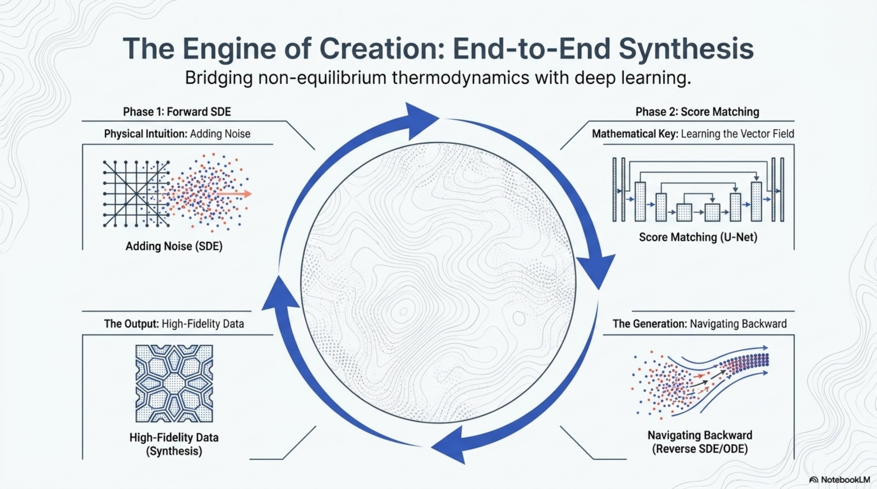
## End-to-end picture
Putting the pieces together:
1. **Forward SDE** $dx = f(x, t)\, dt + g(t)\, dW_t$ smoothly noises clean data into a tractable prior.
2. **Score matching** trains $s_\theta(x, t)$ against the perturbation kernel via the DSM loss — equivalent to noise prediction up to scaling.
3. **Reverse SDE / probability-flow ODE** plugs the trained score back into the dynamics and integrates from $t = T$ to $t = 0$.
4. **Output**: samples drawn from $p_{\text{data}}$, with optional conditioning grafted on by additive scores.
DDPM, DDIM, NCSN, EDM, and modern latent-diffusion text-to-image systems are all instances of this same skeleton with different drift/diffusion choices, parameterizations of $s_\theta$, and ODE/SDE solvers.
## Hands-on companions
Three sections elsewhere in this chapter let you exercise each piece of the framework on a low-dimensional problem you can plot:
* **[Score on a mixture of Gaussians](score-mog-example/score_mog_example)** — derive and visualize $\nabla_x \log p(x)$ for a 2D MoG, then watch Langevin dynamics descend it.
* **[Yang Song's tutorial section](song-tutorial-notebook/Tutorial_on_Score_Based_Generative_Modeling)** — the official MNIST score-SDE walkthrough: VE-SDE, NCSN++, ancestral and Predictor-Corrector samplers, and the probability-flow ODE.
* **[Brownian motion](/aiml-common/lectures/diffusion/brownian-motion/brownian_motion)** — eight trajectories of $dx = g(t)\, dW_t$, the forward SDE in particle form.
* **[DDPM on a 2D MoG](/aiml-common/lectures/diffusion/ddpm/ddpm_mog_tutorial)** — the discrete-time Variance-Preserving instance, with noise prediction.
* **[DDIM on a 2D MoG](/aiml-common/lectures/diffusion/ddim/ddim_mog_tutorial)** — the deterministic ($\eta = 0$) sampler, a first-order discretization of the probability-flow ODE.
## References
1. Song, Sohl-Dickstein, Kingma, Kumar, Ermon, Poole. *Score-Based Generative Modeling through Stochastic Differential Equations.* ICLR 2021. [arxiv.org/abs/2011.13456](https://arxiv.org/abs/2011.13456)
2. Song, Ermon. *Generative Modeling by Estimating Gradients of the Data Distribution.* NeurIPS 2019. [arxiv.org/abs/1907.05600](https://arxiv.org/abs/1907.05600)
3. Vincent. *A Connection Between Score Matching and Denoising Autoencoders.* Neural Computation 2011.
4. Anderson. *Reverse-time diffusion equation models.* Stochastic Processes and their Applications, 1982.
5. Hyvärinen. *Estimation of non-normalized statistical models by score matching.* JMLR 2005.
6. Song, Garg, Shi, Ermon. *Sliced Score Matching: A Scalable Approach to Density and Score Estimation.* UAI 2019. [arxiv.org/abs/1905.07088](https://arxiv.org/abs/1905.07088)
## PyTorch reference
| PyTorch class | Description |
| -------------------------------------------------------------------------------------------------- | -------------------------------------------------------------------------------------------------- |
| [`nn.Conv2d`](https://docs.pytorch.org/docs/2.12/generated/torch.nn.Conv2d.html) | Applies a 2D convolution over an input signal composed of several input planes. |
| [`nn.ConvTranspose2d`](https://docs.pytorch.org/docs/2.12/generated/torch.nn.ConvTranspose2d.html) | Applies a 2D transposed convolution operator over an input image composed of several input planes. |
| [`nn.GroupNorm`](https://docs.pytorch.org/docs/2.12/generated/torch.nn.GroupNorm.html) | Applies Group Normalization over a mini-batch of inputs. |
| [`nn.Linear`](https://docs.pytorch.org/docs/2.12/generated/torch.nn.Linear.html) | Applies an affine linear transformation to the incoming data: $y = xA^T + b$. |
| [`nn.SiLU`](https://docs.pytorch.org/docs/2.12/generated/torch.nn.SiLU.html) | Applies the Sigmoid Linear Unit (SiLU) function, element-wise. |
***
[Edit this page on GitHub](https://github.com/aegean-ai/eaia/edit/main/src/aiml-common/lectures/diffusion/score-based/index.mdx) or [file an issue](https://github.com/aegean-ai/eaia/issues/new/choose).
 ## The intractable wall
 A neural network is a black box from $x \in \mathbb{R}^D$ to a scalar $f_\theta(x) \in \mathbb{R}$. To turn that scalar into a probability density you need
$$
p_\theta(x) \;=\; \frac{\exp(f_\theta(x))}{Z_\theta}, \qquad Z_\theta = \int \exp(f_\theta(x))\, dx.
$$
For images, $D$ is in the tens of thousands. The integral $Z_\theta$ has no closed form and Monte-Carlo estimates are useless at this dimensionality. Every classical likelihood-based generative model — autoregressive, normalizing flows, VAEs — makes some architectural sacrifice to keep $Z_\theta$ tractable: factorize over coordinates, restrict to invertible maps, or optimize a lower bound. Each restriction either limits expressiveness or limits how directly you can score real samples.
The score-based view simply refuses to compute $Z_\theta$.
**Lecture:** open at [≈ 8:00](https://www.youtube.com/watch?v=wMmqCMwuM2Q\&t=480s) for Yang Song's framing of this bottleneck.
## Trade the map for a compass: the score function
A neural network is a black box from $x \in \mathbb{R}^D$ to a scalar $f_\theta(x) \in \mathbb{R}$. To turn that scalar into a probability density you need
$$
p_\theta(x) \;=\; \frac{\exp(f_\theta(x))}{Z_\theta}, \qquad Z_\theta = \int \exp(f_\theta(x))\, dx.
$$
For images, $D$ is in the tens of thousands. The integral $Z_\theta$ has no closed form and Monte-Carlo estimates are useless at this dimensionality. Every classical likelihood-based generative model — autoregressive, normalizing flows, VAEs — makes some architectural sacrifice to keep $Z_\theta$ tractable: factorize over coordinates, restrict to invertible maps, or optimize a lower bound. Each restriction either limits expressiveness or limits how directly you can score real samples.
The score-based view simply refuses to compute $Z_\theta$.
**Lecture:** open at [≈ 8:00](https://www.youtube.com/watch?v=wMmqCMwuM2Q\&t=480s) for Yang Song's framing of this bottleneck.
## Trade the map for a compass: the score function
 Take the gradient of the log of both sides:
$$
s_\theta(x) \;:=\; \nabla_x \log p_\theta(x) \;=\; \nabla_x f_\theta(x) - \cancel{\nabla_x \log Z_\theta} \;=\; \nabla_x f_\theta(x).
$$
The gradient of a constant is zero. The intractable $Z_\theta$ vanishes from the gradient field, and what remains — the **score** — is something a neural network can output directly: a vector field with the same shape as the input.
A density $p(x)$ is a *map* of where probability mass lives. The score $\nabla_x \log p(x)$ is a *compass* that tells you, at any $x$, which direction increases log-density. You don't need the map to navigate: a compass at every point is enough to roll downhill toward the data.
**Lecture:** [≈ 18:00](https://www.youtube.com/watch?v=wMmqCMwuM2Q\&t=1080s).
## The low-density trap
Take the gradient of the log of both sides:
$$
s_\theta(x) \;:=\; \nabla_x \log p_\theta(x) \;=\; \nabla_x f_\theta(x) - \cancel{\nabla_x \log Z_\theta} \;=\; \nabla_x f_\theta(x).
$$
The gradient of a constant is zero. The intractable $Z_\theta$ vanishes from the gradient field, and what remains — the **score** — is something a neural network can output directly: a vector field with the same shape as the input.
A density $p(x)$ is a *map* of where probability mass lives. The score $\nabla_x \log p(x)$ is a *compass* that tells you, at any $x$, which direction increases log-density. You don't need the map to navigate: a compass at every point is enough to roll downhill toward the data.
**Lecture:** [≈ 18:00](https://www.youtube.com/watch?v=wMmqCMwuM2Q\&t=1080s).
## The low-density trap
 Naive score matching has a fatal flaw. Training data $\{x_i\} \sim p_{\text{data}}$ lives on (or near) a thin manifold inside an enormous ambient space. Score matching minimizes the expected squared error between $s_\theta(x)$ and the true score, with the expectation taken **under $p_{\text{data}}$**:
$$
\mathcal{L}(\theta) \;=\; \mathbb{E}_{x \sim p_{\text{data}}}\!\left[\,\bigl\|\, s_\theta(x) - \nabla_x \log p_{\text{data}}(x) \,\bigr\|^2\right].
$$
The model is only trained where the data lives. Far from the manifold the loss puts no weight at all, so the learned compass spins randomly there. At sampling time you start from a Gaussian sample — pure noise, with overwhelming probability *far* from the data — and the compass gives you no signal to follow back. You stay lost.
This is *the* problem the rest of the lecture is built to solve.
**Lecture:** [≈ 36:00](https://www.youtube.com/watch?v=wMmqCMwuM2Q\&t=2160s).
## Noise as a bridge
Naive score matching has a fatal flaw. Training data $\{x_i\} \sim p_{\text{data}}$ lives on (or near) a thin manifold inside an enormous ambient space. Score matching minimizes the expected squared error between $s_\theta(x)$ and the true score, with the expectation taken **under $p_{\text{data}}$**:
$$
\mathcal{L}(\theta) \;=\; \mathbb{E}_{x \sim p_{\text{data}}}\!\left[\,\bigl\|\, s_\theta(x) - \nabla_x \log p_{\text{data}}(x) \,\bigr\|^2\right].
$$
The model is only trained where the data lives. Far from the manifold the loss puts no weight at all, so the learned compass spins randomly there. At sampling time you start from a Gaussian sample — pure noise, with overwhelming probability *far* from the data — and the compass gives you no signal to follow back. You stay lost.
This is *the* problem the rest of the lecture is built to solve.
**Lecture:** [≈ 36:00](https://www.youtube.com/watch?v=wMmqCMwuM2Q\&t=2160s).
## Noise as a bridge
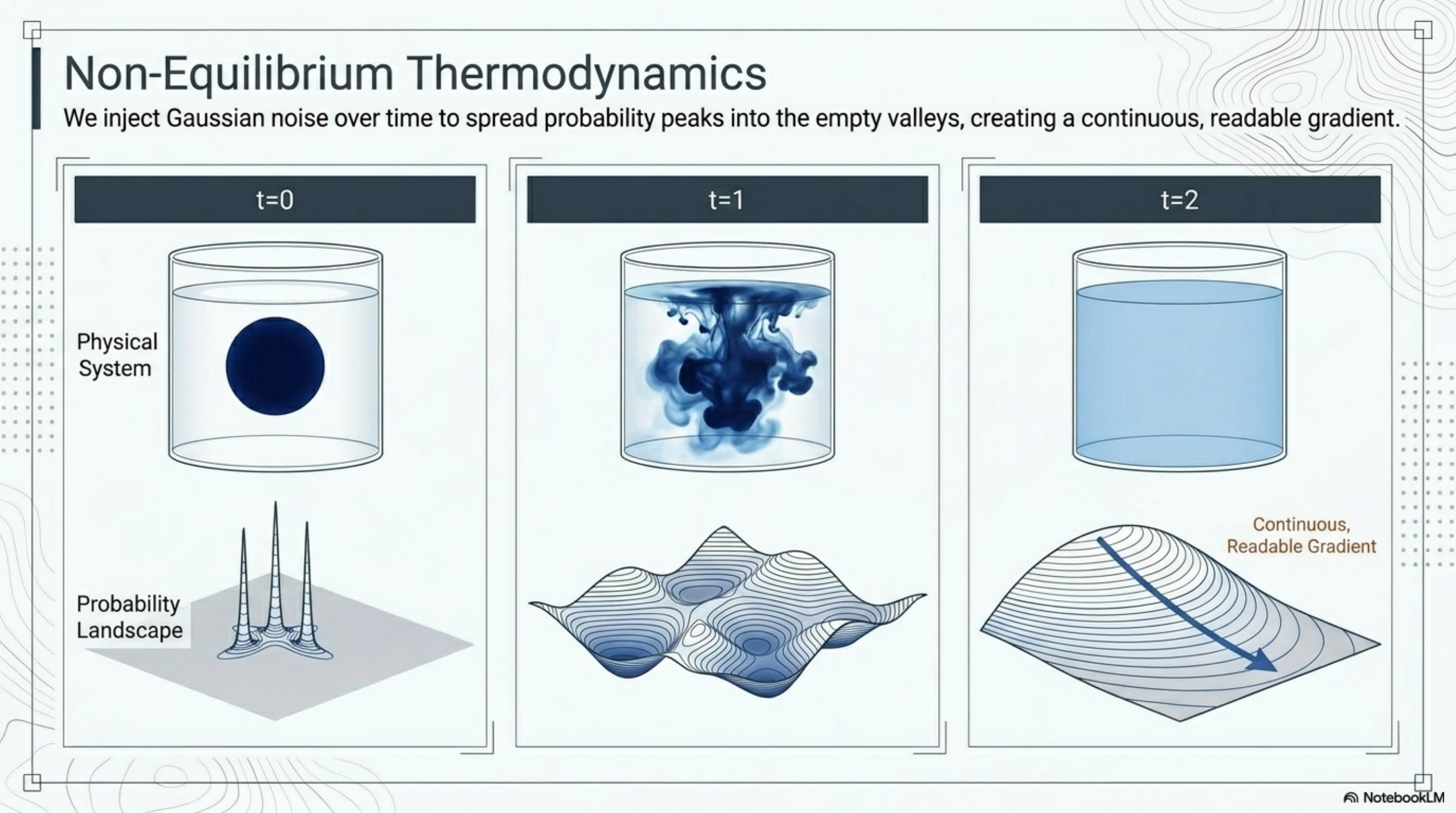 The fix is physical. Inject Gaussian noise into the data and let it spread the probability mass outward over time. Sharp spikes broaden into smooth bumps, empty valleys fill in. After enough noise, the landscape has a non-zero, smoothly-varying gradient *everywhere* — and a network trained to match the score of the noisy distribution will have a well-defined target across the whole space.
This is the non-equilibrium thermodynamics picture: a drop of dye in water starts as a localized concentration ($t=0$) and ends as a uniform mixture ($t \to \infty$). Score-based models reverse that diffusion. The forward process buys you a usable signal across the noise plain; the reverse process trades it back for samples on the data manifold.
This is exactly the [forward noising process](/aiml-common/lectures/diffusion/brownian-motion/brownian_motion) you saw in the Brownian-motion section — eight trajectories spreading from the origin — restated in the language of densities rather than particles.
**Lecture:** [≈ 38:00](https://www.youtube.com/watch?v=wMmqCMwuM2Q\&t=2280s).
## The forward SDE
The fix is physical. Inject Gaussian noise into the data and let it spread the probability mass outward over time. Sharp spikes broaden into smooth bumps, empty valleys fill in. After enough noise, the landscape has a non-zero, smoothly-varying gradient *everywhere* — and a network trained to match the score of the noisy distribution will have a well-defined target across the whole space.
This is the non-equilibrium thermodynamics picture: a drop of dye in water starts as a localized concentration ($t=0$) and ends as a uniform mixture ($t \to \infty$). Score-based models reverse that diffusion. The forward process buys you a usable signal across the noise plain; the reverse process trades it back for samples on the data manifold.
This is exactly the [forward noising process](/aiml-common/lectures/diffusion/brownian-motion/brownian_motion) you saw in the Brownian-motion section — eight trajectories spreading from the origin — restated in the language of densities rather than particles.
**Lecture:** [≈ 38:00](https://www.youtube.com/watch?v=wMmqCMwuM2Q\&t=2280s).
## The forward SDE
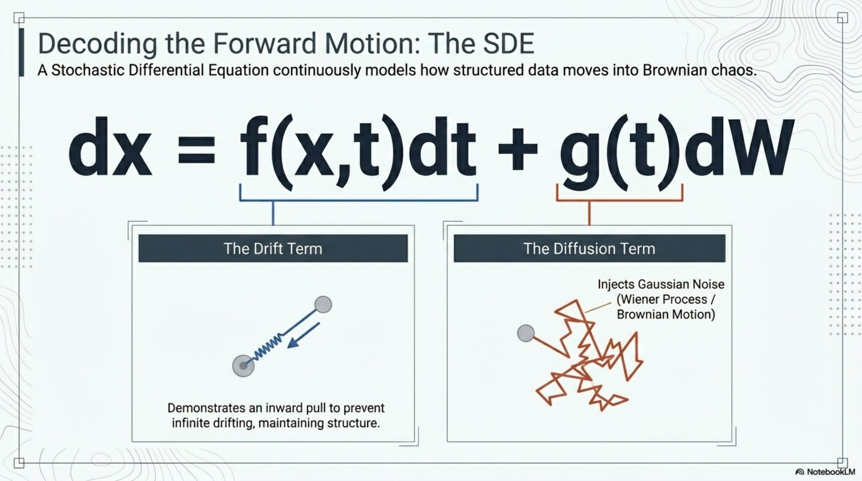 In continuous time the noising process is a stochastic differential equation:
$$
dx \;=\; f(x, t)\, dt \;+\; g(t)\, dW_t, \qquad t \in [0, T],
$$
with $x_0 \sim p_{\text{data}}$ and $W_t$ a standard Wiener process.
* **Drift** $f(x, t)$: a deterministic pull. In Variance-Preserving (VP) SDEs the drift contracts $x$ toward the origin to stop variance from blowing up; in Variance-Exploding (VE) SDEs it is zero.
* **Diffusion** $g(t)$: a scalar volatility schedule controlling how fast Gaussian noise is injected.
DDPM is the **discrete-time Variance-Preserving** instance of this SDE, with the noise schedule $\beta_t$ playing the role of $f$ and $g$. The forward trajectory you trained against in the [DDPM tutorial](/aiml-common/lectures/diffusion/ddpm/ddpm_mog_tutorial) is one Euler-Maruyama discretization of exactly this SDE.
**Lecture:** [≈ 1:00:00](https://www.youtube.com/watch?v=wMmqCMwuM2Q\&t=3600s).
## Training the score network
In continuous time the noising process is a stochastic differential equation:
$$
dx \;=\; f(x, t)\, dt \;+\; g(t)\, dW_t, \qquad t \in [0, T],
$$
with $x_0 \sim p_{\text{data}}$ and $W_t$ a standard Wiener process.
* **Drift** $f(x, t)$: a deterministic pull. In Variance-Preserving (VP) SDEs the drift contracts $x$ toward the origin to stop variance from blowing up; in Variance-Exploding (VE) SDEs it is zero.
* **Diffusion** $g(t)$: a scalar volatility schedule controlling how fast Gaussian noise is injected.
DDPM is the **discrete-time Variance-Preserving** instance of this SDE, with the noise schedule $\beta_t$ playing the role of $f$ and $g$. The forward trajectory you trained against in the [DDPM tutorial](/aiml-common/lectures/diffusion/ddpm/ddpm_mog_tutorial) is one Euler-Maruyama discretization of exactly this SDE.
**Lecture:** [≈ 1:00:00](https://www.youtube.com/watch?v=wMmqCMwuM2Q\&t=3600s).
## Training the score network
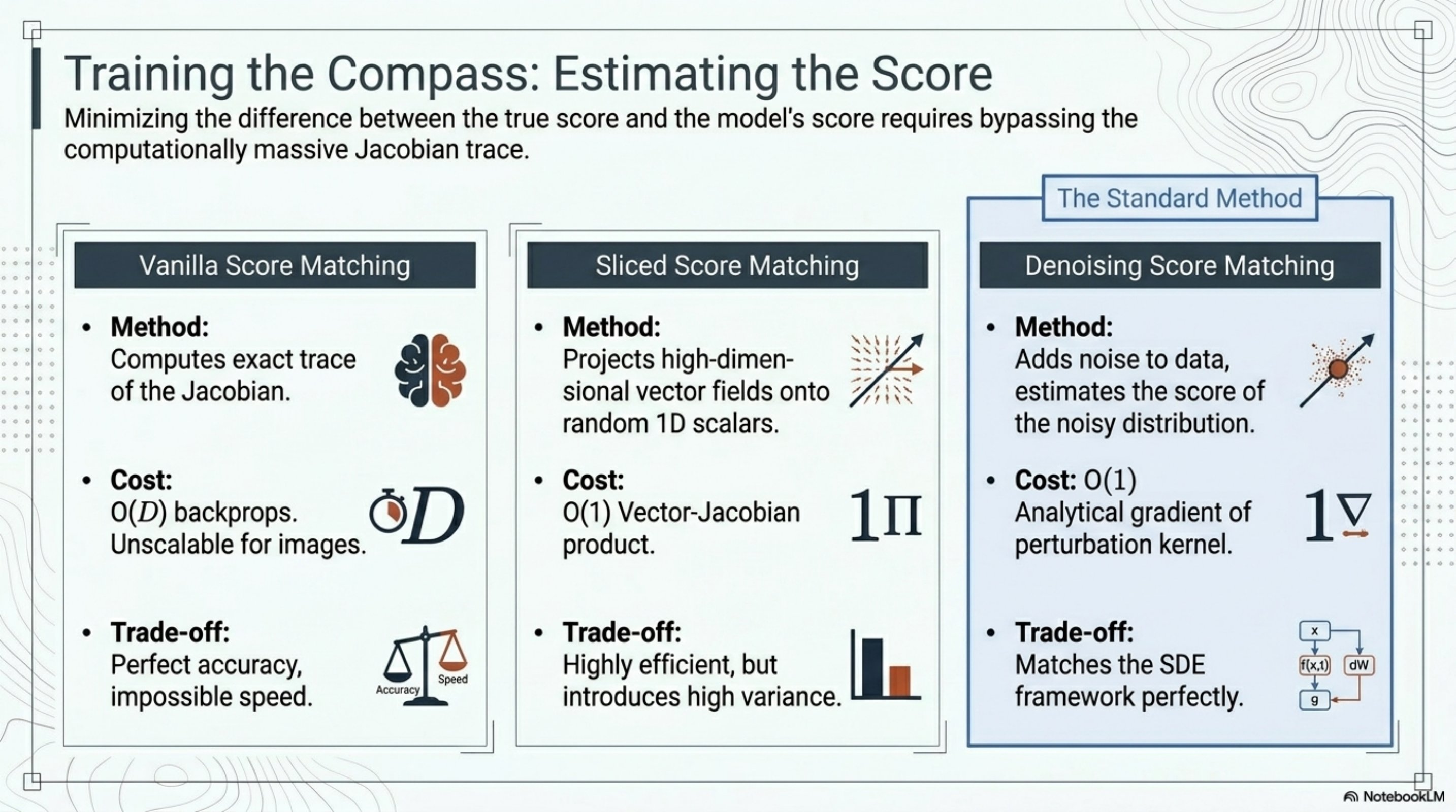 The implicit score-matching loss
$$
\mathbb{E}_{p_{\text{data}}}\!\left[\,\tfrac{1}{2}\|s_\theta(x)\|^2 \;+\; \mathrm{tr}\!\left(\nabla_x s_\theta(x)\right)\right]
$$
removes the unknown $\nabla \log p_{\text{data}}$ via integration by parts, but the Jacobian trace requires $D$ separate backward passes — fatal for images. Three workarounds:
| Variant | Trick | Cost | Trade-off |
| ------------------- | ------------------------------------------------------------------------------------------------------------------------------------------------ | ---------------------------------- | ------------------------------------------------------------- |
| **Vanilla** | Compute $\mathrm{tr}(\nabla s_\theta)$ exactly | $O(D)$ backprops | Exact, unusable above \~1k dims |
| **Sliced** | Random unit vectors $v$; replace trace by $v^\top (\nabla s_\theta)\, v$ | $O(1)$ via Jacobian-vector product | Unbiased, higher variance |
| **Denoising (DSM)** | Perturb $x$ with kernel $q_\sigma(\tilde x \mid x)$; train against the *known* analytic score $\nabla_{\tilde x} \log q_\sigma(\tilde x \mid x)$ | $O(1)$, no Jacobians | Estimates the score of the *noisy* density, not the clean one |
DSM is the standard choice. With Gaussian perturbation $\tilde x = x + \sigma \epsilon, \epsilon \sim \mathcal{N}(0, I)$:
$$
\nabla_{\tilde x} \log q_\sigma(\tilde x \mid x) \;=\; -\frac{\tilde x - x}{\sigma^2} \;=\; -\frac{\epsilon}{\sigma},
$$
so the DSM loss reduces to a re-weighted noise-prediction loss — *this is exactly the DDPM training objective up to a $\sigma$-dependent constant*. The DDPM noise predictor $\epsilon_\theta$ and the score network $s_\theta$ are the same model with a different sign and scale.
**Lecture:** [≈ 22:00–34:00](https://www.youtube.com/watch?v=wMmqCMwuM2Q\&t=1320s) walks through all three variants.
## Reversing the SDE
The implicit score-matching loss
$$
\mathbb{E}_{p_{\text{data}}}\!\left[\,\tfrac{1}{2}\|s_\theta(x)\|^2 \;+\; \mathrm{tr}\!\left(\nabla_x s_\theta(x)\right)\right]
$$
removes the unknown $\nabla \log p_{\text{data}}$ via integration by parts, but the Jacobian trace requires $D$ separate backward passes — fatal for images. Three workarounds:
| Variant | Trick | Cost | Trade-off |
| ------------------- | ------------------------------------------------------------------------------------------------------------------------------------------------ | ---------------------------------- | ------------------------------------------------------------- |
| **Vanilla** | Compute $\mathrm{tr}(\nabla s_\theta)$ exactly | $O(D)$ backprops | Exact, unusable above \~1k dims |
| **Sliced** | Random unit vectors $v$; replace trace by $v^\top (\nabla s_\theta)\, v$ | $O(1)$ via Jacobian-vector product | Unbiased, higher variance |
| **Denoising (DSM)** | Perturb $x$ with kernel $q_\sigma(\tilde x \mid x)$; train against the *known* analytic score $\nabla_{\tilde x} \log q_\sigma(\tilde x \mid x)$ | $O(1)$, no Jacobians | Estimates the score of the *noisy* density, not the clean one |
DSM is the standard choice. With Gaussian perturbation $\tilde x = x + \sigma \epsilon, \epsilon \sim \mathcal{N}(0, I)$:
$$
\nabla_{\tilde x} \log q_\sigma(\tilde x \mid x) \;=\; -\frac{\tilde x - x}{\sigma^2} \;=\; -\frac{\epsilon}{\sigma},
$$
so the DSM loss reduces to a re-weighted noise-prediction loss — *this is exactly the DDPM training objective up to a $\sigma$-dependent constant*. The DDPM noise predictor $\epsilon_\theta$ and the score network $s_\theta$ are the same model with a different sign and scale.
**Lecture:** [≈ 22:00–34:00](https://www.youtube.com/watch?v=wMmqCMwuM2Q\&t=1320s) walks through all three variants.
## Reversing the SDE
![The reverse SDE equation dx = [f(x,t) − g²(t) ∇ log p(x)] dt + g(t) dW̄, with the score term highlighted as 'our trained neural network model'. Below: a curved arrow leading from a noisy random-pixel image on the right back to a clean data sample on the left, with compass icons marking each integration step.](https://mintcdn.com/aegeanaiinc/2VQk5QOBgDu4yUFC/aiml-common/lectures/diffusion/score-based/images/topo-08.png?fit=max&auto=format&n=2VQk5QOBgDu4yUFC&q=85&s=b9b631f46a5c3a1e5d74c05f9ec9205a) Anderson's 1982 reversal theorem is the engine of generation. Every forward diffusion has a reverse-time partner:
$$
dx \;=\; \bigl[\,f(x, t) \;-\; g(t)^2\, \nabla_x \log p_t(x)\,\bigr]\, dt \;+\; g(t)\, d\bar W_t,
$$
where $d\bar W_t$ is a Wiener process running *backward* in time and $p_t$ is the marginal density at time $t$ under the forward SDE.
The only unknown on the right-hand side is $\nabla_x \log p_t(x)$ — and that is precisely what the score network was trained to estimate. Substitute $s_\theta(x, t) \approx \nabla_x \log p_t(x)$ and you have a generator: start from a sample of $p_T \approx \mathcal{N}(0, \sigma_T^2 I)$ and integrate backward to $t = 0$ to land on the data manifold.
This is the same idea as **annealed Langevin dynamics**: at each $t$, take a step downhill along $s_\theta(\cdot, t)$ plus a noise kick, and gradually decrease the noise level. The continuous-time SDE view subsumes the discrete annealed-Langevin sampler used in NCSN and the ancestral sampler used in DDPM.
**Lecture:** [≈ 1:04:00](https://www.youtube.com/watch?v=wMmqCMwuM2Q\&t=3840s).
## Two solvers: stochastic vs deterministic
Anderson's 1982 reversal theorem is the engine of generation. Every forward diffusion has a reverse-time partner:
$$
dx \;=\; \bigl[\,f(x, t) \;-\; g(t)^2\, \nabla_x \log p_t(x)\,\bigr]\, dt \;+\; g(t)\, d\bar W_t,
$$
where $d\bar W_t$ is a Wiener process running *backward* in time and $p_t$ is the marginal density at time $t$ under the forward SDE.
The only unknown on the right-hand side is $\nabla_x \log p_t(x)$ — and that is precisely what the score network was trained to estimate. Substitute $s_\theta(x, t) \approx \nabla_x \log p_t(x)$ and you have a generator: start from a sample of $p_T \approx \mathcal{N}(0, \sigma_T^2 I)$ and integrate backward to $t = 0$ to land on the data manifold.
This is the same idea as **annealed Langevin dynamics**: at each $t$, take a step downhill along $s_\theta(\cdot, t)$ plus a noise kick, and gradually decrease the noise level. The continuous-time SDE view subsumes the discrete annealed-Langevin sampler used in NCSN and the ancestral sampler used in DDPM.
**Lecture:** [≈ 1:04:00](https://www.youtube.com/watch?v=wMmqCMwuM2Q\&t=3840s).
## Two solvers: stochastic vs deterministic
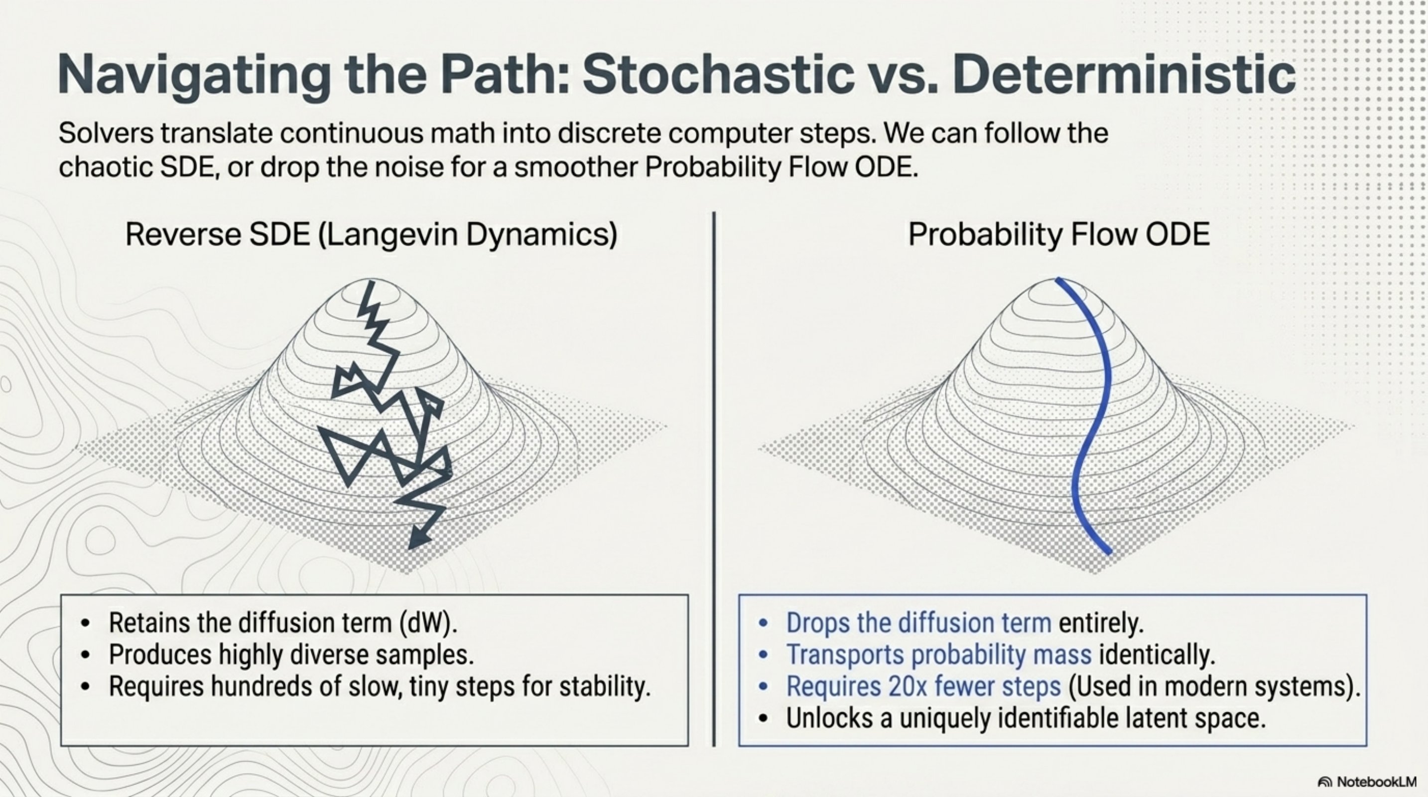 For every score-SDE there is a deterministic ODE that produces *the same marginal densities* $p_t$:
$$
\frac{dx}{dt} \;=\; f(x, t) \;-\; \tfrac{1}{2}\, g(t)^2\, \nabla_x \log p_t(x).
$$
This is the **probability-flow ODE**. The diffusion term is gone — only drift remains — but the family of distributions $\{p_t\}$ swept out by the ODE is identical to the SDE's. Two consequences:
1. **Fewer steps.** ODE solvers (Heun, DPM-Solver, RK45) converge in 20–50 NFEs versus the 500–1000 needed by reverse-SDE samplers. This is what production systems use.
2. **A bijection between data and noise.** The ODE is invertible. Each data point maps to a unique latent code in the prior, which gives you exact log-likelihoods (via the change-of-variables formula and Hutchinson's estimator) and a meaningful semantic latent space — for free, after training.
The deterministic DDIM sampler ($\eta = 0$) you implemented in the [DDIM tutorial](/aiml-common/lectures/diffusion/ddim/ddim_mog_tutorial) is a first-order discretization of this ODE.
**Lecture:** [≈ 1:07:00](https://www.youtube.com/watch?v=wMmqCMwuM2Q\&t=4020s).
## Conditional generation via Bayes' rule
For every score-SDE there is a deterministic ODE that produces *the same marginal densities* $p_t$:
$$
\frac{dx}{dt} \;=\; f(x, t) \;-\; \tfrac{1}{2}\, g(t)^2\, \nabla_x \log p_t(x).
$$
This is the **probability-flow ODE**. The diffusion term is gone — only drift remains — but the family of distributions $\{p_t\}$ swept out by the ODE is identical to the SDE's. Two consequences:
1. **Fewer steps.** ODE solvers (Heun, DPM-Solver, RK45) converge in 20–50 NFEs versus the 500–1000 needed by reverse-SDE samplers. This is what production systems use.
2. **A bijection between data and noise.** The ODE is invertible. Each data point maps to a unique latent code in the prior, which gives you exact log-likelihoods (via the change-of-variables formula and Hutchinson's estimator) and a meaningful semantic latent space — for free, after training.
The deterministic DDIM sampler ($\eta = 0$) you implemented in the [DDIM tutorial](/aiml-common/lectures/diffusion/ddim/ddim_mog_tutorial) is a first-order discretization of this ODE.
**Lecture:** [≈ 1:07:00](https://www.youtube.com/watch?v=wMmqCMwuM2Q\&t=4020s).
## Conditional generation via Bayes' rule
 Conditioning is almost free in score space. Take logs and gradients of Bayes' rule:
$$
\nabla_x \log p(x \mid y) \;=\; \underbrace{\nabla_x \log p(x)}_{\text{unconditional score}} \;+\; \underbrace{\nabla_x \log p(y \mid x)}_{\text{condition / likelihood}}.
$$
The unconditional score is your already-trained diffusion prior. The likelihood term comes from a forward model — a classifier, a degradation operator, a physics simulator. Add the two scores at every step of the reverse SDE/ODE and you sample from the posterior $p(x \mid y)$ without retraining the prior.
This single identity unifies a remarkable range of applications:
* **Inverse problems in medical imaging.** $y$ is a sparse-view CT sinogram; $p(y \mid x)$ is the (linear, known) Radon transform plus measurement noise. The diffusion prior is a generic image model trained once, and the same prior reconstructs MRI, CT, and microscopy images.
* **Class-conditional generation.** $p(y \mid x)$ is a classifier; classifier guidance (and its classifier-free cousin) is the same idea.
* **Text-to-image.** $y$ is a text embedding; the conditional score is approximated jointly with the unconditional one in a single network.
**Lecture:** [≈ 1:14:00](https://www.youtube.com/watch?v=wMmqCMwuM2Q\&t=4440s).
## Where score-based models fit
Conditioning is almost free in score space. Take logs and gradients of Bayes' rule:
$$
\nabla_x \log p(x \mid y) \;=\; \underbrace{\nabla_x \log p(x)}_{\text{unconditional score}} \;+\; \underbrace{\nabla_x \log p(y \mid x)}_{\text{condition / likelihood}}.
$$
The unconditional score is your already-trained diffusion prior. The likelihood term comes from a forward model — a classifier, a degradation operator, a physics simulator. Add the two scores at every step of the reverse SDE/ODE and you sample from the posterior $p(x \mid y)$ without retraining the prior.
This single identity unifies a remarkable range of applications:
* **Inverse problems in medical imaging.** $y$ is a sparse-view CT sinogram; $p(y \mid x)$ is the (linear, known) Radon transform plus measurement noise. The diffusion prior is a generic image model trained once, and the same prior reconstructs MRI, CT, and microscopy images.
* **Class-conditional generation.** $p(y \mid x)$ is a classifier; classifier guidance (and its classifier-free cousin) is the same idea.
* **Text-to-image.** $y$ is a text embedding; the conditional score is approximated jointly with the unconditional one in a single network.
**Lecture:** [≈ 1:14:00](https://www.youtube.com/watch?v=wMmqCMwuM2Q\&t=4440s).
## Where score-based models fit
 The score-SDE framework inherits the strengths of earlier families and shares few of their weaknesses:
* **Sample quality** rivals or exceeds GANs on benchmark image datasets (FID on CIFAR-10, ImageNet, LSUN).
* **Mode coverage** is high: there is no adversary to collapse onto a few easy modes; the loss is a simple regression.
* **Architectural freedom** matches GANs — any network that maps $\mathbb{R}^D \to \mathbb{R}^D$ works as a score model. No invertibility constraint, no encoder-decoder bottleneck.
* **Exact likelihoods** are available via the probability-flow ODE — something GANs cannot offer at all and VAEs only bound.
The trade-off is sampling cost: even with ODE solvers, score-based generation is slower per sample than a single GAN forward pass. Distillation, consistency models, and flow matching are active research directions aimed at closing that gap.
## End-to-end picture
The score-SDE framework inherits the strengths of earlier families and shares few of their weaknesses:
* **Sample quality** rivals or exceeds GANs on benchmark image datasets (FID on CIFAR-10, ImageNet, LSUN).
* **Mode coverage** is high: there is no adversary to collapse onto a few easy modes; the loss is a simple regression.
* **Architectural freedom** matches GANs — any network that maps $\mathbb{R}^D \to \mathbb{R}^D$ works as a score model. No invertibility constraint, no encoder-decoder bottleneck.
* **Exact likelihoods** are available via the probability-flow ODE — something GANs cannot offer at all and VAEs only bound.
The trade-off is sampling cost: even with ODE solvers, score-based generation is slower per sample than a single GAN forward pass. Distillation, consistency models, and flow matching are active research directions aimed at closing that gap.
## End-to-end picture
 Putting the pieces together:
1. **Forward SDE** $dx = f(x, t)\, dt + g(t)\, dW_t$ smoothly noises clean data into a tractable prior.
2. **Score matching** trains $s_\theta(x, t)$ against the perturbation kernel via the DSM loss — equivalent to noise prediction up to scaling.
3. **Reverse SDE / probability-flow ODE** plugs the trained score back into the dynamics and integrates from $t = T$ to $t = 0$.
4. **Output**: samples drawn from $p_{\text{data}}$, with optional conditioning grafted on by additive scores.
DDPM, DDIM, NCSN, EDM, and modern latent-diffusion text-to-image systems are all instances of this same skeleton with different drift/diffusion choices, parameterizations of $s_\theta$, and ODE/SDE solvers.
## Hands-on companions
Three sections elsewhere in this chapter let you exercise each piece of the framework on a low-dimensional problem you can plot:
* **[Score on a mixture of Gaussians](score-mog-example/score_mog_example)** — derive and visualize $\nabla_x \log p(x)$ for a 2D MoG, then watch Langevin dynamics descend it.
* **[Yang Song's tutorial section](song-tutorial-notebook/Tutorial_on_Score_Based_Generative_Modeling)** — the official MNIST score-SDE walkthrough: VE-SDE, NCSN++, ancestral and Predictor-Corrector samplers, and the probability-flow ODE.
* **[Brownian motion](/aiml-common/lectures/diffusion/brownian-motion/brownian_motion)** — eight trajectories of $dx = g(t)\, dW_t$, the forward SDE in particle form.
* **[DDPM on a 2D MoG](/aiml-common/lectures/diffusion/ddpm/ddpm_mog_tutorial)** — the discrete-time Variance-Preserving instance, with noise prediction.
* **[DDIM on a 2D MoG](/aiml-common/lectures/diffusion/ddim/ddim_mog_tutorial)** — the deterministic ($\eta = 0$) sampler, a first-order discretization of the probability-flow ODE.
## References
1. Song, Sohl-Dickstein, Kingma, Kumar, Ermon, Poole. *Score-Based Generative Modeling through Stochastic Differential Equations.* ICLR 2021. [arxiv.org/abs/2011.13456](https://arxiv.org/abs/2011.13456)
2. Song, Ermon. *Generative Modeling by Estimating Gradients of the Data Distribution.* NeurIPS 2019. [arxiv.org/abs/1907.05600](https://arxiv.org/abs/1907.05600)
3. Vincent. *A Connection Between Score Matching and Denoising Autoencoders.* Neural Computation 2011.
4. Anderson. *Reverse-time diffusion equation models.* Stochastic Processes and their Applications, 1982.
5. Hyvärinen. *Estimation of non-normalized statistical models by score matching.* JMLR 2005.
6. Song, Garg, Shi, Ermon. *Sliced Score Matching: A Scalable Approach to Density and Score Estimation.* UAI 2019. [arxiv.org/abs/1905.07088](https://arxiv.org/abs/1905.07088)
## PyTorch reference
| PyTorch class | Description |
| -------------------------------------------------------------------------------------------------- | -------------------------------------------------------------------------------------------------- |
| [`nn.Conv2d`](https://docs.pytorch.org/docs/2.12/generated/torch.nn.Conv2d.html) | Applies a 2D convolution over an input signal composed of several input planes. |
| [`nn.ConvTranspose2d`](https://docs.pytorch.org/docs/2.12/generated/torch.nn.ConvTranspose2d.html) | Applies a 2D transposed convolution operator over an input image composed of several input planes. |
| [`nn.GroupNorm`](https://docs.pytorch.org/docs/2.12/generated/torch.nn.GroupNorm.html) | Applies Group Normalization over a mini-batch of inputs. |
| [`nn.Linear`](https://docs.pytorch.org/docs/2.12/generated/torch.nn.Linear.html) | Applies an affine linear transformation to the incoming data: $y = xA^T + b$. |
| [`nn.SiLU`](https://docs.pytorch.org/docs/2.12/generated/torch.nn.SiLU.html) | Applies the Sigmoid Linear Unit (SiLU) function, element-wise. |
***
Putting the pieces together:
1. **Forward SDE** $dx = f(x, t)\, dt + g(t)\, dW_t$ smoothly noises clean data into a tractable prior.
2. **Score matching** trains $s_\theta(x, t)$ against the perturbation kernel via the DSM loss — equivalent to noise prediction up to scaling.
3. **Reverse SDE / probability-flow ODE** plugs the trained score back into the dynamics and integrates from $t = T$ to $t = 0$.
4. **Output**: samples drawn from $p_{\text{data}}$, with optional conditioning grafted on by additive scores.
DDPM, DDIM, NCSN, EDM, and modern latent-diffusion text-to-image systems are all instances of this same skeleton with different drift/diffusion choices, parameterizations of $s_\theta$, and ODE/SDE solvers.
## Hands-on companions
Three sections elsewhere in this chapter let you exercise each piece of the framework on a low-dimensional problem you can plot:
* **[Score on a mixture of Gaussians](score-mog-example/score_mog_example)** — derive and visualize $\nabla_x \log p(x)$ for a 2D MoG, then watch Langevin dynamics descend it.
* **[Yang Song's tutorial section](song-tutorial-notebook/Tutorial_on_Score_Based_Generative_Modeling)** — the official MNIST score-SDE walkthrough: VE-SDE, NCSN++, ancestral and Predictor-Corrector samplers, and the probability-flow ODE.
* **[Brownian motion](/aiml-common/lectures/diffusion/brownian-motion/brownian_motion)** — eight trajectories of $dx = g(t)\, dW_t$, the forward SDE in particle form.
* **[DDPM on a 2D MoG](/aiml-common/lectures/diffusion/ddpm/ddpm_mog_tutorial)** — the discrete-time Variance-Preserving instance, with noise prediction.
* **[DDIM on a 2D MoG](/aiml-common/lectures/diffusion/ddim/ddim_mog_tutorial)** — the deterministic ($\eta = 0$) sampler, a first-order discretization of the probability-flow ODE.
## References
1. Song, Sohl-Dickstein, Kingma, Kumar, Ermon, Poole. *Score-Based Generative Modeling through Stochastic Differential Equations.* ICLR 2021. [arxiv.org/abs/2011.13456](https://arxiv.org/abs/2011.13456)
2. Song, Ermon. *Generative Modeling by Estimating Gradients of the Data Distribution.* NeurIPS 2019. [arxiv.org/abs/1907.05600](https://arxiv.org/abs/1907.05600)
3. Vincent. *A Connection Between Score Matching and Denoising Autoencoders.* Neural Computation 2011.
4. Anderson. *Reverse-time diffusion equation models.* Stochastic Processes and their Applications, 1982.
5. Hyvärinen. *Estimation of non-normalized statistical models by score matching.* JMLR 2005.
6. Song, Garg, Shi, Ermon. *Sliced Score Matching: A Scalable Approach to Density and Score Estimation.* UAI 2019. [arxiv.org/abs/1905.07088](https://arxiv.org/abs/1905.07088)
## PyTorch reference
| PyTorch class | Description |
| -------------------------------------------------------------------------------------------------- | -------------------------------------------------------------------------------------------------- |
| [`nn.Conv2d`](https://docs.pytorch.org/docs/2.12/generated/torch.nn.Conv2d.html) | Applies a 2D convolution over an input signal composed of several input planes. |
| [`nn.ConvTranspose2d`](https://docs.pytorch.org/docs/2.12/generated/torch.nn.ConvTranspose2d.html) | Applies a 2D transposed convolution operator over an input image composed of several input planes. |
| [`nn.GroupNorm`](https://docs.pytorch.org/docs/2.12/generated/torch.nn.GroupNorm.html) | Applies Group Normalization over a mini-batch of inputs. |
| [`nn.Linear`](https://docs.pytorch.org/docs/2.12/generated/torch.nn.Linear.html) | Applies an affine linear transformation to the incoming data: $y = xA^T + b$. |
| [`nn.SiLU`](https://docs.pytorch.org/docs/2.12/generated/torch.nn.SiLU.html) | Applies the Sigmoid Linear Unit (SiLU) function, element-wise. |
***