> ## Documentation Index
> Fetch the complete documentation index at: https://aegean.ai/llms.txt
> Use this file to discover all available pages before exploring further.
# Score MoG Example
> Score-based generative modeling on a 2D Mixture of Gaussians.
 ## The target distribution
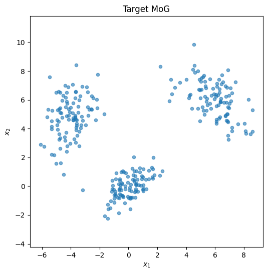
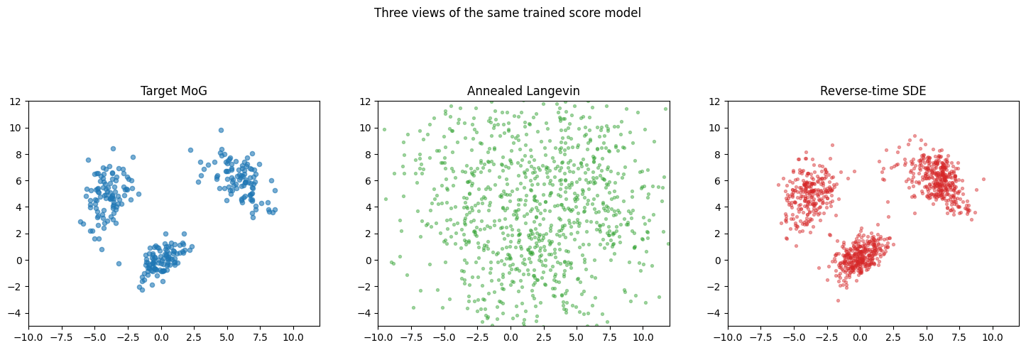
The same 2D Mixture of Gaussians used by the [DDPM](/aiml-common/lectures/diffusion/ddpm/ddpm_mog_tutorial), [DDIM](/aiml-common/lectures/diffusion/ddim/ddim_mog_tutorial), and [Brownian motion](/aiml-common/lectures/diffusion/brownian-motion/brownian_motion) tutorials: three anisotropic Gaussians, seed 42, 300 points total. To DDPM you trained a noise predictor $\epsilon_\theta$. Here you train a **score predictor** $s_\theta(x, \sigma)$ that approximates $\nabla_x \log p_\sigma(x)$, the gradient of the log-density of the data after Gaussian smoothing at scale $\sigma$.
```python theme={null}
import numpy as np
import torch
import torch.nn as nn
import torch.nn.functional as F
import matplotlib.pyplot as plt
torch.manual_seed(42)
np.random.seed(42)
device = torch.device("cuda" if torch.cuda.is_available() else "cpu")
n_samples = 300
components = [
{"mean": np.array([0.0, 0.0]), "cov": np.array([[1.0, 0.5], [0.5, 1.0]])},
{"mean": np.array([6.0, 6.0]), "cov": np.array([[1.5, -0.7], [-0.7, 1.5]])},
{"mean": np.array([-4.0, 5.0]), "cov": np.array([[0.8, 0.0], [0.0, 2.0]])},
]
weights = np.array([1.0, 1.0, 1.0]) / 3.0
rng = np.random.default_rng(42)
data_np = np.vstack([
rng.multivariate_normal(c["mean"], c["cov"], n_samples // 3) for c in components
]).astype(np.float32)
data = torch.from_numpy(data_np).to(device)
```
## The target distribution
The same 2D Mixture of Gaussians used by the [DDPM](/aiml-common/lectures/diffusion/ddpm/ddpm_mog_tutorial), [DDIM](/aiml-common/lectures/diffusion/ddim/ddim_mog_tutorial), and [Brownian motion](/aiml-common/lectures/diffusion/brownian-motion/brownian_motion) tutorials: three anisotropic Gaussians, seed 42, 300 points total. To DDPM you trained a noise predictor $\epsilon_\theta$. Here you train a **score predictor** $s_\theta(x, \sigma)$ that approximates $\nabla_x \log p_\sigma(x)$, the gradient of the log-density of the data after Gaussian smoothing at scale $\sigma$.
```python theme={null}
import numpy as np
import torch
import torch.nn as nn
import torch.nn.functional as F
import matplotlib.pyplot as plt
torch.manual_seed(42)
np.random.seed(42)
device = torch.device("cuda" if torch.cuda.is_available() else "cpu")
n_samples = 300
components = [
{"mean": np.array([0.0, 0.0]), "cov": np.array([[1.0, 0.5], [0.5, 1.0]])},
{"mean": np.array([6.0, 6.0]), "cov": np.array([[1.5, -0.7], [-0.7, 1.5]])},
{"mean": np.array([-4.0, 5.0]), "cov": np.array([[0.8, 0.0], [0.0, 2.0]])},
]
weights = np.array([1.0, 1.0, 1.0]) / 3.0
rng = np.random.default_rng(42)
data_np = np.vstack([
rng.multivariate_normal(c["mean"], c["cov"], n_samples // 3) for c in components
]).astype(np.float32)
data = torch.from_numpy(data_np).to(device)
```
 ## Denoising score matching
We perturb data with Gaussian noise at scale $\sigma$:
$\tilde x = x + \sigma\, \epsilon, \qquad \epsilon \sim \mathcal{N}(0, I)$
The score of the smoothed density satisfies
$\nabla_{\tilde x} \log p_\sigma(\tilde x \mid x) = -\frac{\tilde x - x}{\sigma^2} = -\frac{\epsilon}{\sigma}$
so the **denoising score-matching** objective
$L = \mathbb{E}_{x, \sigma, \epsilon}\!\left[\,\sigma^2 \big\| s_\theta(\tilde x, \sigma) + \epsilon / \sigma \big\|^2\,\right]$
trains $s_\theta(\tilde x, \sigma)$ to estimate $\nabla \log p_\sigma(\tilde x)$ across a range of noise scales. The $\sigma^2$ weighting makes the loss balanced across scales, Song & Ermon 2019.
We use a logarithmic noise schedule $\sigma \in [\sigma_{\min}, \sigma_{\max}]$ with $\sigma_{\min} = 0.05$, $\sigma_{\max} = 5.0$.
```python theme={null}
SIGMA_MIN, SIGMA_MAX = 0.05, 5.0
def sample_sigma(n):
"""Log-uniform sample of sigma for DSM training."""
u = torch.rand(n, device=device)
return SIGMA_MIN * (SIGMA_MAX / SIGMA_MIN) ** u
class ScoreNet(nn.Module):
"""Small MLP s_theta(x, sigma). Conditions on log(sigma) via sinusoidal embedding."""
def __init__(self, sigma_dim=64, hidden=128):
super().__init__()
self.sigma_dim = sigma_dim
self.net = nn.Sequential(
nn.Linear(2 + sigma_dim, hidden), nn.SiLU(),
nn.Linear(hidden, hidden), nn.SiLU(),
nn.Linear(hidden, hidden), nn.SiLU(),
nn.Linear(hidden, 2),
)
def sigma_emb(self, sigma):
half = self.sigma_dim // 2
freqs = torch.exp(-np.log(10000) * torch.arange(half, device=sigma.device) / half)
emb = torch.log(sigma).unsqueeze(-1) * freqs
return torch.cat([emb.sin(), emb.cos()], dim=-1)
def forward(self, x, sigma):
return self.net(torch.cat([x, self.sigma_emb(sigma)], dim=-1))
model = ScoreNet().to(device)
optim = torch.optim.Adam(model.parameters(), lr=2e-3)
```
## Training
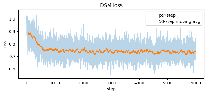
Standard DSM loop: sample a batch, sample a per-example $\sigma$, perturb, predict the score, minimize the noise-conditional loss.
```python theme={null}
batch_size = 256
n_steps = 6000
losses = []
for step in range(n_steps):
idx = torch.randint(0, data.shape[0], (batch_size,), device=device)
x0 = data[idx]
sigma = sample_sigma(batch_size)
eps = torch.randn_like(x0)
xt = x0 + sigma.unsqueeze(-1) * eps
target = -eps / sigma.unsqueeze(-1)
pred = model(xt, sigma)
loss = ((sigma.unsqueeze(-1) * (pred - target)) ** 2).mean()
optim.zero_grad(); loss.backward(); optim.step()
losses.append(loss.item())
if (step + 1) % 1500 == 0:
print(f"step {step + 1:>5d} loss {float(np.mean(losses[-500:])):.4f}")
print("trained.")
```
```output theme={null}
step 1500 loss 0.7443
```
```output theme={null}
step 3000 loss 0.7404
```
```output theme={null}
step 4500 loss 0.7398
```
```output theme={null}
step 6000 loss 0.7311
trained.
```
## Denoising score matching
We perturb data with Gaussian noise at scale $\sigma$:
$\tilde x = x + \sigma\, \epsilon, \qquad \epsilon \sim \mathcal{N}(0, I)$
The score of the smoothed density satisfies
$\nabla_{\tilde x} \log p_\sigma(\tilde x \mid x) = -\frac{\tilde x - x}{\sigma^2} = -\frac{\epsilon}{\sigma}$
so the **denoising score-matching** objective
$L = \mathbb{E}_{x, \sigma, \epsilon}\!\left[\,\sigma^2 \big\| s_\theta(\tilde x, \sigma) + \epsilon / \sigma \big\|^2\,\right]$
trains $s_\theta(\tilde x, \sigma)$ to estimate $\nabla \log p_\sigma(\tilde x)$ across a range of noise scales. The $\sigma^2$ weighting makes the loss balanced across scales, Song & Ermon 2019.
We use a logarithmic noise schedule $\sigma \in [\sigma_{\min}, \sigma_{\max}]$ with $\sigma_{\min} = 0.05$, $\sigma_{\max} = 5.0$.
```python theme={null}
SIGMA_MIN, SIGMA_MAX = 0.05, 5.0
def sample_sigma(n):
"""Log-uniform sample of sigma for DSM training."""
u = torch.rand(n, device=device)
return SIGMA_MIN * (SIGMA_MAX / SIGMA_MIN) ** u
class ScoreNet(nn.Module):
"""Small MLP s_theta(x, sigma). Conditions on log(sigma) via sinusoidal embedding."""
def __init__(self, sigma_dim=64, hidden=128):
super().__init__()
self.sigma_dim = sigma_dim
self.net = nn.Sequential(
nn.Linear(2 + sigma_dim, hidden), nn.SiLU(),
nn.Linear(hidden, hidden), nn.SiLU(),
nn.Linear(hidden, hidden), nn.SiLU(),
nn.Linear(hidden, 2),
)
def sigma_emb(self, sigma):
half = self.sigma_dim // 2
freqs = torch.exp(-np.log(10000) * torch.arange(half, device=sigma.device) / half)
emb = torch.log(sigma).unsqueeze(-1) * freqs
return torch.cat([emb.sin(), emb.cos()], dim=-1)
def forward(self, x, sigma):
return self.net(torch.cat([x, self.sigma_emb(sigma)], dim=-1))
model = ScoreNet().to(device)
optim = torch.optim.Adam(model.parameters(), lr=2e-3)
```
## Training
Standard DSM loop: sample a batch, sample a per-example $\sigma$, perturb, predict the score, minimize the noise-conditional loss.
```python theme={null}
batch_size = 256
n_steps = 6000
losses = []
for step in range(n_steps):
idx = torch.randint(0, data.shape[0], (batch_size,), device=device)
x0 = data[idx]
sigma = sample_sigma(batch_size)
eps = torch.randn_like(x0)
xt = x0 + sigma.unsqueeze(-1) * eps
target = -eps / sigma.unsqueeze(-1)
pred = model(xt, sigma)
loss = ((sigma.unsqueeze(-1) * (pred - target)) ** 2).mean()
optim.zero_grad(); loss.backward(); optim.step()
losses.append(loss.item())
if (step + 1) % 1500 == 0:
print(f"step {step + 1:>5d} loss {float(np.mean(losses[-500:])):.4f}")
print("trained.")
```
```output theme={null}
step 1500 loss 0.7443
```
```output theme={null}
step 3000 loss 0.7404
```
```output theme={null}
step 4500 loss 0.7398
```
```output theme={null}
step 6000 loss 0.7311
trained.
```
 ## The learned score field
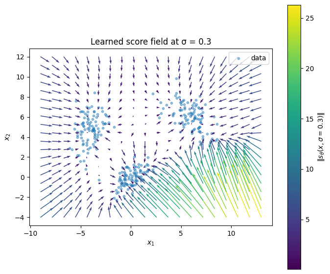
Evaluate $s_\theta$ on a grid at low noise ($\sigma = 0.3$), at this scale the score points toward the data manifold, so the field should converge into the three MoG modes.
```python theme={null}
@torch.no_grad()
def score_grid(sigma_val=0.3, lo=(-9, -4), hi=(13, 12), n=20):
xs = torch.linspace(lo[0], hi[0], n, device=device)
ys = torch.linspace(lo[1], hi[1], n, device=device)
X, Y = torch.meshgrid(xs, ys, indexing="xy")
pts = torch.stack([X.flatten(), Y.flatten()], dim=-1)
sigma = torch.full((pts.shape[0],), sigma_val, device=device)
s = model(pts, sigma)
return X.cpu().numpy(), Y.cpu().numpy(), s[:, 0].view(n, n).cpu().numpy(), s[:, 1].view(n, n).cpu().numpy()
X, Y, U, V = score_grid()
```
## The learned score field
Evaluate $s_\theta$ on a grid at low noise ($\sigma = 0.3$), at this scale the score points toward the data manifold, so the field should converge into the three MoG modes.
```python theme={null}
@torch.no_grad()
def score_grid(sigma_val=0.3, lo=(-9, -4), hi=(13, 12), n=20):
xs = torch.linspace(lo[0], hi[0], n, device=device)
ys = torch.linspace(lo[1], hi[1], n, device=device)
X, Y = torch.meshgrid(xs, ys, indexing="xy")
pts = torch.stack([X.flatten(), Y.flatten()], dim=-1)
sigma = torch.full((pts.shape[0],), sigma_val, device=device)
s = model(pts, sigma)
return X.cpu().numpy(), Y.cpu().numpy(), s[:, 0].view(n, n).cpu().numpy(), s[:, 1].view(n, n).cpu().numpy()
X, Y, U, V = score_grid()
```
 *Above: the analytical score field $\nabla \log p(x)$ for this MoG, manimgl-rendered. Compare with the matplotlib quiver of the **learned** $s_\theta$, both should pull mass toward the three component centers.*
## Annealed Langevin sampling
Generate samples by running Langevin dynamics at decreasing noise levels:
$x_{k+1} = x_k + \alpha_k\, s_\theta(x_k, \sigma_k) + \sqrt{2\alpha_k}\, z_k, \quad z_k \sim \mathcal{N}(0, I)$
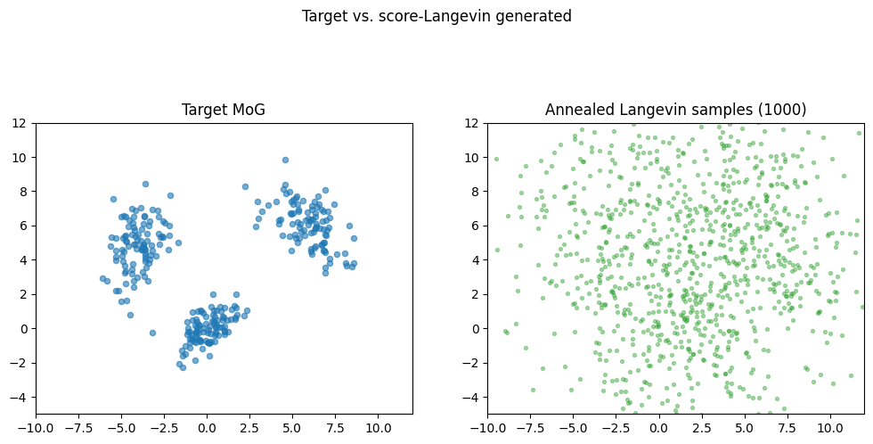
with step size $\alpha_k = \epsilon \cdot \sigma_k^2 / \sigma_{\min}^2$, Song & Ermon's recipe. Larger $\sigma$ steps cover broad regions of space; smaller $\sigma$ steps refine onto the data manifold.
```python theme={null}
@torch.no_grad()
def annealed_langevin(n=1000, n_sigmas=10, n_inner=8, eps=2e-5):
sigmas = torch.from_numpy(
np.geomspace(SIGMA_MAX, SIGMA_MIN, n_sigmas).astype(np.float32)
).to(device)
x = torch.randn(n, 2, device=device) * SIGMA_MAX + torch.tensor([2.0, 4.0], device=device)
for sigma in sigmas:
alpha = eps * (sigma ** 2) / (SIGMA_MIN ** 2)
sigma_b = sigma.expand(n)
for _ in range(n_inner):
s = model(x, sigma_b)
x = x + alpha * s + torch.sqrt(2 * alpha) * torch.randn_like(x)
return x.cpu().numpy()
samples_langevin = annealed_langevin(n=1000)
```
*Above: 80 particles released uniformly, then annealed-Langevin-stepped through a geometric noise schedule from $\sigma = 2.5$ down to $\sigma = 0.15$. The cloud condenses into the three MoG components.*
*Above: the analytical score field $\nabla \log p(x)$ for this MoG, manimgl-rendered. Compare with the matplotlib quiver of the **learned** $s_\theta$, both should pull mass toward the three component centers.*
## Annealed Langevin sampling
Generate samples by running Langevin dynamics at decreasing noise levels:
$x_{k+1} = x_k + \alpha_k\, s_\theta(x_k, \sigma_k) + \sqrt{2\alpha_k}\, z_k, \quad z_k \sim \mathcal{N}(0, I)$
with step size $\alpha_k = \epsilon \cdot \sigma_k^2 / \sigma_{\min}^2$, Song & Ermon's recipe. Larger $\sigma$ steps cover broad regions of space; smaller $\sigma$ steps refine onto the data manifold.
```python theme={null}
@torch.no_grad()
def annealed_langevin(n=1000, n_sigmas=10, n_inner=8, eps=2e-5):
sigmas = torch.from_numpy(
np.geomspace(SIGMA_MAX, SIGMA_MIN, n_sigmas).astype(np.float32)
).to(device)
x = torch.randn(n, 2, device=device) * SIGMA_MAX + torch.tensor([2.0, 4.0], device=device)
for sigma in sigmas:
alpha = eps * (sigma ** 2) / (SIGMA_MIN ** 2)
sigma_b = sigma.expand(n)
for _ in range(n_inner):
s = model(x, sigma_b)
x = x + alpha * s + torch.sqrt(2 * alpha) * torch.randn_like(x)
return x.cpu().numpy()
samples_langevin = annealed_langevin(n=1000)
```
*Above: 80 particles released uniformly, then annealed-Langevin-stepped through a geometric noise schedule from $\sigma = 2.5$ down to $\sigma = 0.15$. The cloud condenses into the three MoG components.*
 ## Reverse-time SDE
The variance-exploding (VE) SDE has forward $dx_t = \sqrt{\frac{d[\sigma_t^2]}{dt}}\, dW_t$ and reverse-time form
$dx_t = -\frac{d[\sigma_t^2]}{dt}\, s_\theta(x_t, \sigma_t)\, dt + \sqrt{\frac{d[\sigma_t^2]}{dt}}\, d\bar W_t$
Discretize with Euler-Maruyama from $t = 1$ down to $t = 0$. This is the same chain as DDIM at $\eta = 1$ in the score-SDE framework.
```python theme={null}
@torch.no_grad()
def reverse_sde(n=1000, n_steps=400):
"""Euler-Maruyama on the reverse VE-SDE with learned score."""
ts = torch.linspace(1.0, 0.0, n_steps + 1, device=device)
sigmas = SIGMA_MIN * (SIGMA_MAX / SIGMA_MIN) ** ts
x = torch.randn(n, 2, device=device) * sigmas[0] + torch.tensor([2.0, 4.0], device=device)
for i in range(n_steps):
sigma = sigmas[i]
sigma_next = sigmas[i + 1]
# d[sigma^2] over this Δt is sigma^2 - sigma_next^2 (positive going forward in time)
d_sigma2 = (sigma ** 2 - sigma_next ** 2).clamp(min=0)
sigma_b = sigma.expand(n)
s = model(x, sigma_b)
x = x + d_sigma2 * s + torch.sqrt(d_sigma2) * torch.randn_like(x)
return x.cpu().numpy()
samples_sde = reverse_sde(n=1000)
```
*Above: 60 particles seeded broadly, evolving under the reverse-time SDE driven by the analytical MoG score. Trails show each particle's path as it condenses into one of the three modes.*
## Reverse-time SDE
The variance-exploding (VE) SDE has forward $dx_t = \sqrt{\frac{d[\sigma_t^2]}{dt}}\, dW_t$ and reverse-time form
$dx_t = -\frac{d[\sigma_t^2]}{dt}\, s_\theta(x_t, \sigma_t)\, dt + \sqrt{\frac{d[\sigma_t^2]}{dt}}\, d\bar W_t$
Discretize with Euler-Maruyama from $t = 1$ down to $t = 0$. This is the same chain as DDIM at $\eta = 1$ in the score-SDE framework.
```python theme={null}
@torch.no_grad()
def reverse_sde(n=1000, n_steps=400):
"""Euler-Maruyama on the reverse VE-SDE with learned score."""
ts = torch.linspace(1.0, 0.0, n_steps + 1, device=device)
sigmas = SIGMA_MIN * (SIGMA_MAX / SIGMA_MIN) ** ts
x = torch.randn(n, 2, device=device) * sigmas[0] + torch.tensor([2.0, 4.0], device=device)
for i in range(n_steps):
sigma = sigmas[i]
sigma_next = sigmas[i + 1]
# d[sigma^2] over this Δt is sigma^2 - sigma_next^2 (positive going forward in time)
d_sigma2 = (sigma ** 2 - sigma_next ** 2).clamp(min=0)
sigma_b = sigma.expand(n)
s = model(x, sigma_b)
x = x + d_sigma2 * s + torch.sqrt(d_sigma2) * torch.randn_like(x)
return x.cpu().numpy()
samples_sde = reverse_sde(n=1000)
```
*Above: 60 particles seeded broadly, evolving under the reverse-time SDE driven by the analytical MoG score. Trails show each particle's path as it condenses into one of the three modes.*
 ## Connections to other concepts
* **Score-matching is the unifying view.** DDPM's noise predictor $\epsilon_\theta$ is, up to the scaling $-1/\sigma$, a score predictor; DDIM's deterministic sampler is the probability-flow ODE limit of the same score-SDE. The framework above subsumes both.
* **Sampler decoupling.** Once you have $s_\theta$, you can swap samplers: annealed Langevin, reverse SDE, probability-flow ODE, predictor-corrector. The trained network is unchanged.
* **The information-theoretic angle.** $s_\theta(x, t)$ is the local geometry of $\log p_t(x)$, the same quantity that, integrated through Fisher-information identities, gives mutual information bounds. See [AURA-672](https://aegean-ai.atlassian.net/browse/AURA-672) for the score → Fisher → MI thread.
## References
1. Song, Ermon. *Generative Modeling by Estimating Gradients of the Data Distribution.* NeurIPS 2019. [arxiv.org/abs/1907.05600](https://arxiv.org/abs/1907.05600)
2. Song, Sohl-Dickstein, Kingma, Kumar, Ermon, Poole. *Score-Based Generative Modeling through Stochastic Differential Equations.* ICLR 2021. [arxiv.org/abs/2011.13456](https://arxiv.org/abs/2011.13456)
3. Vincent. *A Connection Between Score Matching and Denoising Autoencoders.* Neural Computation 2011.
## PyTorch reference
| PyTorch class | Description |
| ---------------------------------------------------------------------------------------- | ----------------------------------------------------------------------------- |
| [`nn.Sequential`](https://docs.pytorch.org/docs/2.12/generated/torch.nn.Sequential.html) | A sequential container. |
| [`nn.Linear`](https://docs.pytorch.org/docs/2.12/generated/torch.nn.Linear.html) | Applies an affine linear transformation to the incoming data: $y = xA^T + b$. |
| [`nn.SiLU`](https://docs.pytorch.org/docs/2.12/generated/torch.nn.SiLU.html) | Applies the Sigmoid Linear Unit (SiLU) function, element-wise. |
***
[Edit this page on GitHub](https://github.com/aegean-ai/eaia/edit/main/src/aiml-common/lectures/diffusion/score-based/score-mog-example/score_mog_example.mdx) or [file an issue](https://github.com/aegean-ai/eaia/issues/new/choose).
## Connections to other concepts
* **Score-matching is the unifying view.** DDPM's noise predictor $\epsilon_\theta$ is, up to the scaling $-1/\sigma$, a score predictor; DDIM's deterministic sampler is the probability-flow ODE limit of the same score-SDE. The framework above subsumes both.
* **Sampler decoupling.** Once you have $s_\theta$, you can swap samplers: annealed Langevin, reverse SDE, probability-flow ODE, predictor-corrector. The trained network is unchanged.
* **The information-theoretic angle.** $s_\theta(x, t)$ is the local geometry of $\log p_t(x)$, the same quantity that, integrated through Fisher-information identities, gives mutual information bounds. See [AURA-672](https://aegean-ai.atlassian.net/browse/AURA-672) for the score → Fisher → MI thread.
## References
1. Song, Ermon. *Generative Modeling by Estimating Gradients of the Data Distribution.* NeurIPS 2019. [arxiv.org/abs/1907.05600](https://arxiv.org/abs/1907.05600)
2. Song, Sohl-Dickstein, Kingma, Kumar, Ermon, Poole. *Score-Based Generative Modeling through Stochastic Differential Equations.* ICLR 2021. [arxiv.org/abs/2011.13456](https://arxiv.org/abs/2011.13456)
3. Vincent. *A Connection Between Score Matching and Denoising Autoencoders.* Neural Computation 2011.
## PyTorch reference
| PyTorch class | Description |
| ---------------------------------------------------------------------------------------- | ----------------------------------------------------------------------------- |
| [`nn.Sequential`](https://docs.pytorch.org/docs/2.12/generated/torch.nn.Sequential.html) | A sequential container. |
| [`nn.Linear`](https://docs.pytorch.org/docs/2.12/generated/torch.nn.Linear.html) | Applies an affine linear transformation to the incoming data: $y = xA^T + b$. |
| [`nn.SiLU`](https://docs.pytorch.org/docs/2.12/generated/torch.nn.SiLU.html) | Applies the Sigmoid Linear Unit (SiLU) function, element-wise. |
***
[Edit this page on GitHub](https://github.com/aegean-ai/eaia/edit/main/src/aiml-common/lectures/diffusion/score-based/score-mog-example/score_mog_example.mdx) or [file an issue](https://github.com/aegean-ai/eaia/issues/new/choose).