> ## Documentation Index
> Fetch the complete documentation index at: https://aegean.ai/llms.txt
> Use this file to discover all available pages before exploring further.
# Empirical and expected risk
> Understanding the bias-variance tradeoff and generalization error in machine learning models.
Let $p_{\text{data}}(\boldsymbol{x}, y)$ denote the (unknown) true data-generating distribution; all training and test points are drawn i.i.d. from it. A training set $\mathbb{X} = \{(\boldsymbol{x}^{(j)},\, y^{(j)})\}_{j=1}^m$ induces the **empirical distribution**
$\hat{p}_{\text{data}}(\boldsymbol{x}, y) \;=\; \frac{1}{m}\sum_{j=1}^{m} \delta_{(\boldsymbol{x}^{(j)},\, y^{(j)})}(\boldsymbol{x}, y)$
— the uniform discrete distribution placing mass $1/m$ on each observed sample. The predictor is $\hat{y} = g(\boldsymbol{x};\, \boldsymbol{\theta})$. The **empirical risk** and the **expected risk** are then the same expected squared error under two different distributions:
$R_{\text{emp}}(\boldsymbol{\theta}) \;=\; \mathbb{E}_{(\boldsymbol{x},y) \sim \hat{p}_{\text{data}}}\!\left[(g(\boldsymbol{x};\,\boldsymbol{\theta}) - y)^2\right] \;=\; \frac{1}{m}\sum_{j=1}^{m} \big(g(\boldsymbol{x}^{(j)};\,\boldsymbol{\theta}) - y^{(j)}\big)^2$
$R(\boldsymbol{\theta}) \;=\; \mathbb{E}_{(\boldsymbol{x},y) \sim p_{\text{data}}}\!\left[(g(\boldsymbol{x};\,\boldsymbol{\theta}) - y)^2\right]$
$R_{\text{emp}}$ is a finite-sample plug-in for $R$: deterministic once $\mathbb{X}$ is fixed, but random *across* draws of $\mathbb{X}$, because $\hat{p}_{\text{data}}$ itself is random.
When we examine the MSE at a fixed test point $(\boldsymbol{x}^{(i)},\, y^{(i)})$ and decompose it into bias and variance, we are asking how the predictor $\hat{y}^{(i)} = g(\boldsymbol{x}^{(i)};\, \boldsymbol{\theta})$ varies under re-draws of $\mathbb{X}$. The fitted parameters $\boldsymbol{\theta} = \boldsymbol{\theta}(\hat{p}_{\text{data}})$ are random because $\hat{p}_{\text{data}}$ is, and that randomness flows through to $\hat{y}^{(i)}$. Strictly,
$\mathbb{E}_{\boldsymbol{\theta}}[\,\cdot\,] \;=\; \mathbb{E}_{\mathbb{X}}\!\big[\,\cdot\,(\boldsymbol{\theta}(\hat{p}_{\text{data}}))\big]$
so the subscript $\boldsymbol{\theta}$ is shorthand for "average over realizations of $\hat{p}_{\text{data}}$ induced by drawing $\mathbb{X}$ i.i.d. from $p_{\text{data}}$". The bias and variance terms measure properties of the *learning procedure*, not of any one trained model: bias is the average error of the procedure across draws of $\hat{p}_{\text{data}}$, and variance is how much its predictions move when $\hat{p}_{\text{data}}$ shifts under a new $\mathbb{X}$.
Because $p_{\text{data}}$ is unknown in practice, $\mathbb{E}_{\mathbb{X}}$ is never computed exactly. We approximate it by bootstrap resampling, cross-validation, or running the same training pipeline with different random seeds on disjoint splits.
The mean squared error of the predictor at the test point, averaged over training-set draws, is
$\mathrm{MSE} \;=\; \mathbb{E}_{\boldsymbol{\theta}}\!\left[(\hat{y}^{(i)} - y^{(i)})^2\right]$
and the central result of the next section is that it splits cleanly into a bias and a variance contribution:
$\mathrm{MSE} \;=\; \mathrm{Bias}_{\boldsymbol{\theta}}(\hat{y}^{(i)})^2 + \mathrm{Var}_{\boldsymbol{\theta}}(\hat{y}^{(i)})$
## Derivation of the bias-variance decomposition
Throughout the derivation, treat $y^{(i)}$ as fixed and let all randomness sit in $\boldsymbol{\theta}(\hat{p}_{\text{data}})$ (equivalently, in $\mathbb{X}$). Define
$\mathrm{Bias}_{\boldsymbol{\theta}}(\hat{y}^{(i)}) = \mathbb{E}_{\boldsymbol{\theta}}[\hat{y}^{(i)}] - y^{(i)}, \qquad \mathrm{Var}_{\boldsymbol{\theta}}(\hat{y}^{(i)}) = \mathbb{E}_{\boldsymbol{\theta}}\!\left[(\hat{y}^{(i)} - \mathbb{E}_{\boldsymbol{\theta}}[\hat{y}^{(i)}])^2\right]$
Add and subtract $\mathbb{E}_{\boldsymbol{\theta}}[\hat{y}^{(i)}]$ inside the squared error:
$\mathrm{MSE} = \mathbb{E}_{\boldsymbol{\theta}}\!\left[\big(\hat{y}^{(i)} - \mathbb{E}_{\boldsymbol{\theta}}[\hat{y}^{(i)}] + \mathbb{E}_{\boldsymbol{\theta}}[\hat{y}^{(i)}] - y^{(i)}\big)^2\right]$
Expand the square:
$= \mathbb{E}_{\boldsymbol{\theta}}\!\left[(\hat{y}^{(i)} - \mathbb{E}_{\boldsymbol{\theta}}[\hat{y}^{(i)}])^2 + 2(\hat{y}^{(i)} - \mathbb{E}_{\boldsymbol{\theta}}[\hat{y}^{(i)}])(\mathbb{E}_{\boldsymbol{\theta}}[\hat{y}^{(i)}] - y^{(i)}) + (\mathbb{E}_{\boldsymbol{\theta}}[\hat{y}^{(i)}] - y^{(i)})^2\right]$
By linearity of expectation, and pulling the constant factor $(\mathbb{E}_{\boldsymbol{\theta}}[\hat{y}^{(i)}] - y^{(i)})$ out of the cross term:
$= \underbrace{\mathbb{E}_{\boldsymbol{\theta}}\!\left[(\hat{y}^{(i)} - \mathbb{E}_{\boldsymbol{\theta}}[\hat{y}^{(i)}])^2\right]}_{\mathrm{Var}_{\boldsymbol{\theta}}(\hat{y}^{(i)})} + 2(\mathbb{E}_{\boldsymbol{\theta}}[\hat{y}^{(i)}] - y^{(i)})\,\mathbb{E}_{\boldsymbol{\theta}}\!\left[\hat{y}^{(i)} - \mathbb{E}_{\boldsymbol{\theta}}[\hat{y}^{(i)}]\right] + \underbrace{(\mathbb{E}_{\boldsymbol{\theta}}[\hat{y}^{(i)}] - y^{(i)})^2}_{\mathrm{Bias}_{\boldsymbol{\theta}}(\hat{y}^{(i)})^2}$
The cross term vanishes because the inner deviation has zero mean:
$\mathbb{E}_{\boldsymbol{\theta}}\!\left[\hat{y}^{(i)} - \mathbb{E}_{\boldsymbol{\theta}}[\hat{y}^{(i)}]\right] = \mathbb{E}_{\boldsymbol{\theta}}[\hat{y}^{(i)}] - \mathbb{E}_{\boldsymbol{\theta}}[\hat{y}^{(i)}] = 0$
leaving the bias-variance decomposition stated above:
$\mathrm{MSE} = \mathrm{Bias}_{\boldsymbol{\theta}}(\hat{y}^{(i)})^2 + \mathrm{Var}_{\boldsymbol{\theta}}(\hat{y}^{(i)})$
The derivation follows the standard estimator-MSE argument from [Wikipedia](https://en.wikipedia.org/wiki/Mean_squared_error), specialized to the prediction setting where the estimator is the model's output $\hat{y}^{(i)}$. Note that this form assumes the target $y^{(i)}$ is deterministic; if $y^{(i)}$ itself carries irreducible noise $\varepsilon$ with variance $\sigma^2$, the decomposition gains an additive term and becomes $\mathrm{Bias}^2 + \mathrm{Var} + \sigma^2$.
## Interpretation
The decomposition splits the prediction error into two competing sources and as shown in the plots above, increasing model capacity can really increase the variance of $\hat{y}$. We have seen that as $\boldsymbol{\theta}$ is fit to exactly match, or memorize, the data, it minimizes the bias (in fact for model complexity $M=9$ the bias is 0) but it also exhibits significant variability that is itself translated to $\hat{y}$. Although the definition of model *capacity* is far more rigorous, we will broadly associate complexity with capacity and borrow the figure below from Ian Goodfellow's book to demonstrate the tradeoff between bias and variance. What we have done with regularization is to find the $\lambda$ that minimizes generalization error, i.e., find the optimal model capacity.
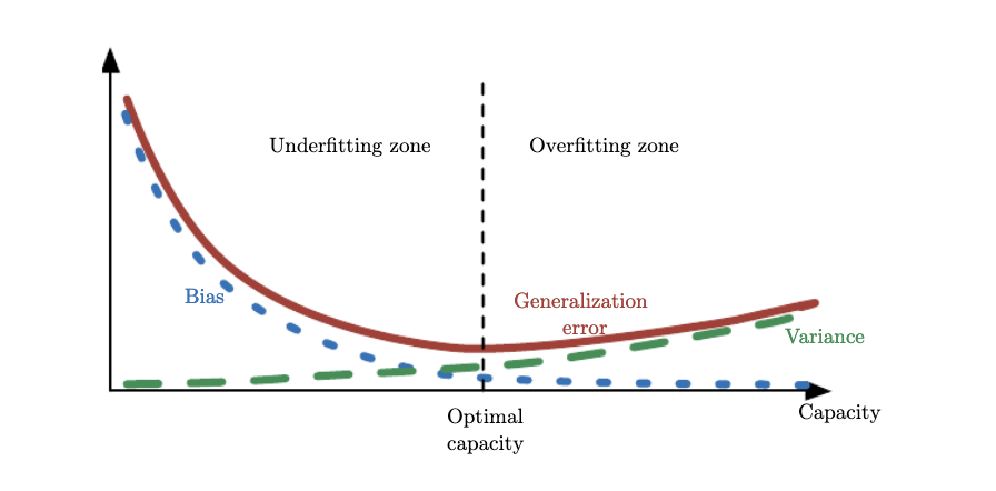 *As capacity increases (x-axis), bias (dotted) tends to decrease and variance (dashed) tends to increase, yielding another U-shaped curve for generalization error (bold curve). If we vary capacity along one axis, there is an optimal capacity, with underfitting when the capacity is below this optimum and overfitting when it is above.*
## Bias and Variance Decomposition during the training process
Apart from the composition of the generalization error for various model capacities, it is interesting to make some general comments regarding the decomposition of the generalization error (also known as empirical risk) during training. Early in training the bias is large because the predictor output is far from the target function. The variance is very small because the data has had little influence yet. Late in training the bias is small because the predictor has learned the underlying function. However if train for too long then the predictor will also have learned the noise specific to the dataset (overfitting). In such case the variance will be large because the noise varies between training and test datasets.
**Do not extrapolate the U-shaped curve above to highly over-parameterized models.** Modern over-parameterized neural networks empirically exhibit a *double descent* risk curve (Belkin et al., 2018; Nakkiran et al., 2019): as capacity grows past the interpolation threshold, the test error first rises (classical regime) and then *falls* again in the over-parameterized regime, sometimes below the optimum of the classical U-curve. The bias-variance picture above remains a good guide in the under-parameterized regime that this page focuses on, but cannot predict generalization behavior of contemporary deep models.
*As capacity increases (x-axis), bias (dotted) tends to decrease and variance (dashed) tends to increase, yielding another U-shaped curve for generalization error (bold curve). If we vary capacity along one axis, there is an optimal capacity, with underfitting when the capacity is below this optimum and overfitting when it is above.*
## Bias and Variance Decomposition during the training process
Apart from the composition of the generalization error for various model capacities, it is interesting to make some general comments regarding the decomposition of the generalization error (also known as empirical risk) during training. Early in training the bias is large because the predictor output is far from the target function. The variance is very small because the data has had little influence yet. Late in training the bias is small because the predictor has learned the underlying function. However if train for too long then the predictor will also have learned the noise specific to the dataset (overfitting). In such case the variance will be large because the noise varies between training and test datasets.
**Do not extrapolate the U-shaped curve above to highly over-parameterized models.** Modern over-parameterized neural networks empirically exhibit a *double descent* risk curve (Belkin et al., 2018; Nakkiran et al., 2019): as capacity grows past the interpolation threshold, the test error first rises (classical regime) and then *falls* again in the over-parameterized regime, sometimes below the optimum of the classical U-curve. The bias-variance picture above remains a good guide in the under-parameterized regime that this page focuses on, but cannot predict generalization behavior of contemporary deep models.
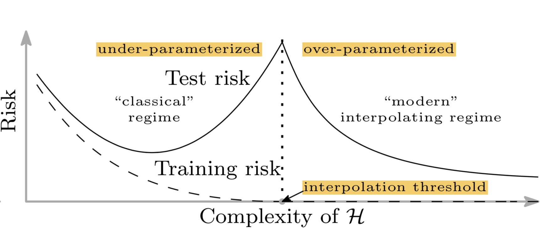 *Past the interpolation threshold, the test error can drop again — the "double descent" phenomenon.*
## References
* Belkin, M., Hsu, D., Ma, S., Mandal, S. (2018). *Reconciling modern machine learning practice and the bias-variance trade-off*.
* Nakkiran, P., Kaplun, G., Kalimeris, D., Yang, T., Edelman, B., et al. (2019). *SGD on neural networks learns functions of increasing complexity*.
***
[Edit this page on GitHub](https://github.com/aegean-ai/eaia/edit/main/src/aiml-common/lectures/empirical-risk/index.mdx) or [file an issue](https://github.com/aegean-ai/eaia/issues/new/choose).
*Past the interpolation threshold, the test error can drop again — the "double descent" phenomenon.*
## References
* Belkin, M., Hsu, D., Ma, S., Mandal, S. (2018). *Reconciling modern machine learning practice and the bias-variance trade-off*.
* Nakkiran, P., Kaplun, G., Kalimeris, D., Yang, T., Edelman, B., et al. (2019). *SGD on neural networks learns functions of increasing complexity*.
***
[Edit this page on GitHub](https://github.com/aegean-ai/eaia/edit/main/src/aiml-common/lectures/empirical-risk/index.mdx) or [file an issue](https://github.com/aegean-ai/eaia/issues/new/choose).