> ## Documentation Index
> Fetch the complete documentation index at: https://aegean.ai/llms.txt
> Use this file to discover all available pages before exploring further.
# Smoothing an Image with Blur Filters
> Box, Gaussian, and binomial blur filters, their frequency responses, and why the binomial cancels the checkerboard.
 *This section was written by [Kaushik Kachireddy](https://github.com/kaushik0x7d2) ([pull request #76](https://github.com/pantelis/eng-ai-agents/pull/76)), with help from an AI coding agent (Claude Code) on the code. It reproduces the ideas of Chapter 17 of [*Foundations of Computer Vision*](https://visionbook.mit.edu/blurring_2.html) by Antonio Torralba, Phillip Isola, and William T. Freeman. The book's own figures are not reproduced here, because the book's license covers only the work in full; links point to them instead.*
Blur filters are **low-pass** linear filters: they attenuate high spatial frequencies (fine detail and noise) while preserving the low-frequency structure of an image. This section builds the three filter families of the book's chapter, the **box filter**, the **Gaussian filter**, and the **binomial filter**, implements each as a convolution, and regenerates the figures from the underlying math.
Four of the book's figures (17.1, 17.4, 17.5, and 17.8) are built on its own photographs. Here the same experiments run on scikit-image test images, and each links to the book's version.
```python theme={null}
import numpy as np
import torch
import torch.nn.functional as F
import matplotlib.pyplot as plt
from PIL import Image
from skimage import data, img_as_float
from skimage.color import rgb2gray
_ = torch.manual_seed(0)
np.random.seed(0)
torch.set_default_dtype(torch.float32)
plt.rcParams.update({
"figure.dpi": 130,
"savefig.dpi": 130,
"image.cmap": "gray",
"image.interpolation": "nearest",
"axes.grid": False,
})
# Grayscale sample image, float32 in [0, 1].
IMG = torch.from_numpy(img_as_float(data.camera())).float() # 512x512 'cameraman'
H, W = IMG.shape
```
**Images replaced for licensing.** The book is published under a CC BY-NC-ND license, which covers only the book as a whole and not its individual images, so this page does not republish the book's photographs. License-free images stand in for them:
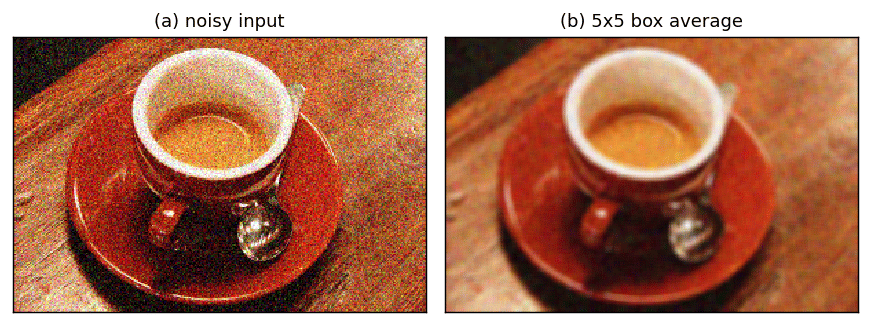
* The *coffee* photograph with added noise (scikit-image) stands in for [a noisy photograph of a stop sign (Figure 17.1)](https://visionbook.mit.edu/figures/blur_filters/stop_256_noise_3.jpg).
* The *cameraman* photograph blurred to sigma=2 (scikit-image) stands in for [a photograph of a zebra blurred to sigma=2 (Figure 17.4)](https://visionbook.mit.edu/figures/spatial_filters/gausian_zebra_c_2.jpg).
* A block portrait built from the *astronaut* photograph (scikit-image) stands in for [Harmon and Julesz's block portrait of Lincoln (Figure 17.5)](https://visionbook.mit.edu/figures/blur_filters/Jules_Lincoln_1971.jpg).
* The *coffee* photograph (scikit-image) stands in for [a photograph of a boat (Figure 17.8)](https://visionbook.mit.edu/figures/blur_filters/boat_d_binomial.jpg).
If you use the book for non-commercial purposes, you can swap the originals back in: each line that loads a stand-in carries the original's link in a comment.
```python theme={null}
def conv2d(image, kernel, mode='reflect'):
"""2D convolution, "same" size, reflect-padded.
Kernels here are symmetric, so convolution == cross-correlation; the kernel is
still flipped for correctness. `kernel` is expected to be DC-normalized (sums to 1)
when a brightness-preserving blur is wanted.
"""
k = torch.as_tensor(kernel, dtype=torch.float32).flip(0).flip(1)
kh, kw = k.shape
x = F.pad(image[None, None], (kw // 2, kw // 2, kh // 2, kh // 2), mode=mode)
return F.conv2d(x, k[None, None])[0, 0]
def conv2d_rgb(image, kernel, mode='reflect'):
"""Apply the same 2D kernel to each channel of an (H, W, 3) color image."""
return torch.stack([conv2d(image[..., c], kernel, mode) for c in range(3)], dim=-1)
```
## Noise removal versus detail loss
A blur filter replaces each pixel with a **weighted average of its neighbors**. Averaging suppresses zero-mean noise, because the fluctuations cancel, but it also smears genuine high-frequency detail. That is the central tradeoff of the whole chapter. Figure 17.1 makes it visible: additive noise is largely gone after a $5\times5$ average, at the cost of sharpness. The book uses a [noisy photograph of a stop sign](https://visionbook.mit.edu/blurring_2.html#fig-stop_256_noise_3); here noise is added to a color test photograph.
```python theme={null}
# Figure 17.1: a noisy color photo, denoised by a box average.
# The image has 3 channels; the box is applied to each (R, G, B) independently.
# stand-in for a noisy photograph of a stop sign in the book; original: https://visionbook.mit.edu/figures/blur_filters/stop_256_noise_3.jpg
clean = F.avg_pool2d(torch.from_numpy(img_as_float(data.coffee())).float().permute(2, 0, 1)[None], 2)[0].permute(1, 2, 0)
stop_noisy = (clean + 0.12 * torch.randn_like(clean)).clamp(0, 1) # additive Gaussian noise
avg5 = torch.ones(5, 5) / 25.0 # normalized 5x5 box (DC gain = 1)
denoised = conv2d_rgb(stop_noisy, avg5)
```
*This section was written by [Kaushik Kachireddy](https://github.com/kaushik0x7d2) ([pull request #76](https://github.com/pantelis/eng-ai-agents/pull/76)), with help from an AI coding agent (Claude Code) on the code. It reproduces the ideas of Chapter 17 of [*Foundations of Computer Vision*](https://visionbook.mit.edu/blurring_2.html) by Antonio Torralba, Phillip Isola, and William T. Freeman. The book's own figures are not reproduced here, because the book's license covers only the work in full; links point to them instead.*
Blur filters are **low-pass** linear filters: they attenuate high spatial frequencies (fine detail and noise) while preserving the low-frequency structure of an image. This section builds the three filter families of the book's chapter, the **box filter**, the **Gaussian filter**, and the **binomial filter**, implements each as a convolution, and regenerates the figures from the underlying math.
Four of the book's figures (17.1, 17.4, 17.5, and 17.8) are built on its own photographs. Here the same experiments run on scikit-image test images, and each links to the book's version.
```python theme={null}
import numpy as np
import torch
import torch.nn.functional as F
import matplotlib.pyplot as plt
from PIL import Image
from skimage import data, img_as_float
from skimage.color import rgb2gray
_ = torch.manual_seed(0)
np.random.seed(0)
torch.set_default_dtype(torch.float32)
plt.rcParams.update({
"figure.dpi": 130,
"savefig.dpi": 130,
"image.cmap": "gray",
"image.interpolation": "nearest",
"axes.grid": False,
})
# Grayscale sample image, float32 in [0, 1].
IMG = torch.from_numpy(img_as_float(data.camera())).float() # 512x512 'cameraman'
H, W = IMG.shape
```
**Images replaced for licensing.** The book is published under a CC BY-NC-ND license, which covers only the book as a whole and not its individual images, so this page does not republish the book's photographs. License-free images stand in for them:
* The *coffee* photograph with added noise (scikit-image) stands in for [a noisy photograph of a stop sign (Figure 17.1)](https://visionbook.mit.edu/figures/blur_filters/stop_256_noise_3.jpg).
* The *cameraman* photograph blurred to sigma=2 (scikit-image) stands in for [a photograph of a zebra blurred to sigma=2 (Figure 17.4)](https://visionbook.mit.edu/figures/spatial_filters/gausian_zebra_c_2.jpg).
* A block portrait built from the *astronaut* photograph (scikit-image) stands in for [Harmon and Julesz's block portrait of Lincoln (Figure 17.5)](https://visionbook.mit.edu/figures/blur_filters/Jules_Lincoln_1971.jpg).
* The *coffee* photograph (scikit-image) stands in for [a photograph of a boat (Figure 17.8)](https://visionbook.mit.edu/figures/blur_filters/boat_d_binomial.jpg).
If you use the book for non-commercial purposes, you can swap the originals back in: each line that loads a stand-in carries the original's link in a comment.
```python theme={null}
def conv2d(image, kernel, mode='reflect'):
"""2D convolution, "same" size, reflect-padded.
Kernels here are symmetric, so convolution == cross-correlation; the kernel is
still flipped for correctness. `kernel` is expected to be DC-normalized (sums to 1)
when a brightness-preserving blur is wanted.
"""
k = torch.as_tensor(kernel, dtype=torch.float32).flip(0).flip(1)
kh, kw = k.shape
x = F.pad(image[None, None], (kw // 2, kw // 2, kh // 2, kh // 2), mode=mode)
return F.conv2d(x, k[None, None])[0, 0]
def conv2d_rgb(image, kernel, mode='reflect'):
"""Apply the same 2D kernel to each channel of an (H, W, 3) color image."""
return torch.stack([conv2d(image[..., c], kernel, mode) for c in range(3)], dim=-1)
```
## Noise removal versus detail loss
A blur filter replaces each pixel with a **weighted average of its neighbors**. Averaging suppresses zero-mean noise, because the fluctuations cancel, but it also smears genuine high-frequency detail. That is the central tradeoff of the whole chapter. Figure 17.1 makes it visible: additive noise is largely gone after a $5\times5$ average, at the cost of sharpness. The book uses a [noisy photograph of a stop sign](https://visionbook.mit.edu/blurring_2.html#fig-stop_256_noise_3); here noise is added to a color test photograph.
```python theme={null}
# Figure 17.1: a noisy color photo, denoised by a box average.
# The image has 3 channels; the box is applied to each (R, G, B) independently.
# stand-in for a noisy photograph of a stop sign in the book; original: https://visionbook.mit.edu/figures/blur_filters/stop_256_noise_3.jpg
clean = F.avg_pool2d(torch.from_numpy(img_as_float(data.coffee())).float().permute(2, 0, 1)[None], 2)[0].permute(1, 2, 0)
stop_noisy = (clean + 0.12 * torch.randn_like(clean)).clamp(0, 1) # additive Gaussian noise
avg5 = torch.ones(5, 5) / 25.0 # normalized 5x5 box (DC gain = 1)
denoised = conv2d_rgb(stop_noisy, avg5)
```
 ```python theme={null}
print('input std (noisy):', stop_noisy.std().item())
print('output std (blurred):', denoised.std().item(),
' # lower = high-frequency noise attenuated')
```
```output theme={null}
input std (noisy): 0.2977954149246216
output std (blurred): 0.26855558156967163 # lower = high-frequency noise attenuated
```
## The box filter
The 2D **box** (moving-average) kernel keeps a constant weight inside a rectangular window and zero outside:
$\mathrm{box}_{N,M}[n,m] = \begin{cases}1 & -N \le n \le N,\ -M \le m \le M\\ 0 & \text{otherwise}\end{cases}$
To keep average brightness unchanged the kernel must have **DC gain 1**, i.e. its coefficients sum to 1, so you divide by $(2N+1)(2M+1)$.
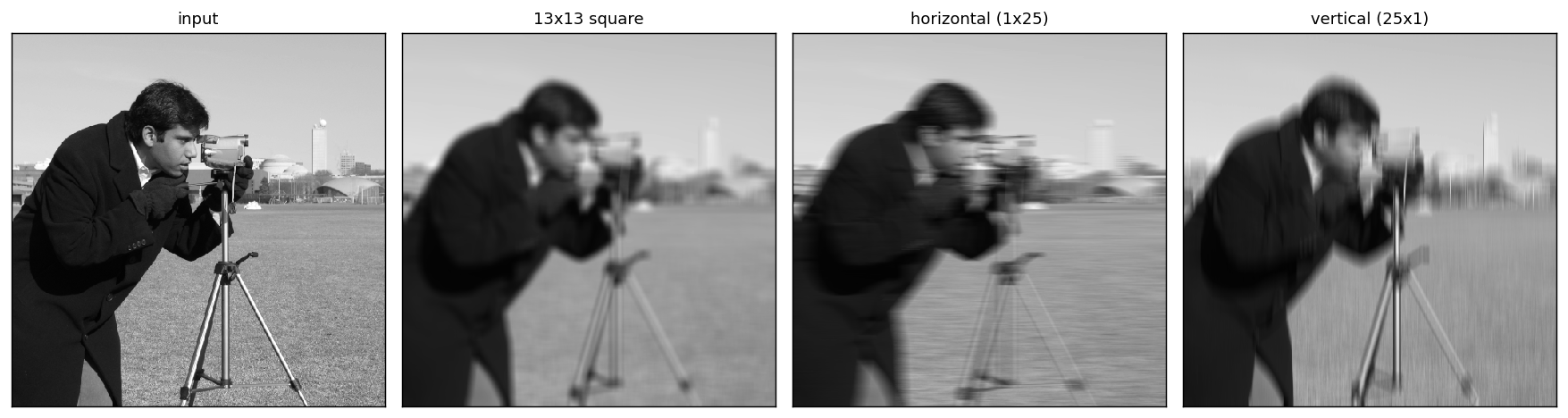
The box is **separable**: $\mathrm{box}_{N,M} = \mathrm{box}_N^{\,x} * \mathrm{box}_M^{\,y}$, a full-window rectangle equals a horizontal bar convolved with a vertical bar. Choosing $N=0$ or $M=0$ blurs along a single axis, as the middle and right panels of Figure 17.2 show.
```python theme={null}
# Figure 17.2: square vs horizontal vs vertical box blur.
def box_kernel(N, M):
return torch.ones(2 * N + 1, 2 * M + 1) / ((2 * N + 1) * (2 * M + 1))
square = conv2d(IMG, box_kernel(6, 6)) # 13x13 window
horiz = conv2d(IMG, box_kernel(0, 12)) # 1x25 -> blurs horizontally
vert = conv2d(IMG, box_kernel(12, 0)) # 25x1 -> blurs vertically
```
```python theme={null}
print('input std (noisy):', stop_noisy.std().item())
print('output std (blurred):', denoised.std().item(),
' # lower = high-frequency noise attenuated')
```
```output theme={null}
input std (noisy): 0.2977954149246216
output std (blurred): 0.26855558156967163 # lower = high-frequency noise attenuated
```
## The box filter
The 2D **box** (moving-average) kernel keeps a constant weight inside a rectangular window and zero outside:
$\mathrm{box}_{N,M}[n,m] = \begin{cases}1 & -N \le n \le N,\ -M \le m \le M\\ 0 & \text{otherwise}\end{cases}$
To keep average brightness unchanged the kernel must have **DC gain 1**, i.e. its coefficients sum to 1, so you divide by $(2N+1)(2M+1)$.
The box is **separable**: $\mathrm{box}_{N,M} = \mathrm{box}_N^{\,x} * \mathrm{box}_M^{\,y}$, a full-window rectangle equals a horizontal bar convolved with a vertical bar. Choosing $N=0$ or $M=0$ blurs along a single axis, as the middle and right panels of Figure 17.2 show.
```python theme={null}
# Figure 17.2: square vs horizontal vs vertical box blur.
def box_kernel(N, M):
return torch.ones(2 * N + 1, 2 * M + 1) / ((2 * N + 1) * (2 * M + 1))
square = conv2d(IMG, box_kernel(6, 6)) # 13x13 window
horiz = conv2d(IMG, box_kernel(0, 12)) # 1x25 -> blurs horizontally
vert = conv2d(IMG, box_kernel(12, 0)) # 25x1 -> blurs vertically
```
 ```python theme={null}
# Separability check: 2D box == 1D-x then 1D-y.
sep = conv2d(conv2d(IMG, box_kernel(0, 6)), box_kernel(6, 0))
print('max |2D-box - separable|:', (square - sep).abs().max().item())
```
```output theme={null}
max |2D-box - separable|: 1.8477439880371094e-06
```
### The box filter's frequency response is not monotonic
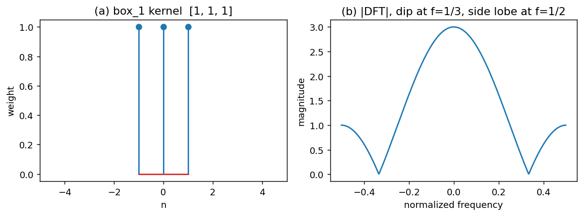
The discrete-time Fourier transform of a length-$L$ box is a **Dirichlet (aliased-sinc) kernel**. Because a sinc oscillates, the box's frequency response has **side lobes**: some high frequencies are passed with *more* gain than lower ones, and the sign flips lobe-to-lobe. A good low-pass filter should instead fall off monotonically. That is the motivation for the Gaussian and binomial filters below.
```python theme={null}
# Figure 17.3: the book's box_1 = [1, 1, 1] kernel and its (rippled) Fourier
# magnitude. |Box_1(w)| = |1 + 2 cos(w)| dips to 0 at f=1/3 then rises again to a
# side lobe at f=1/2, non-monotonic, unlike the Gaussian/binomial.
box1d = np.array([1.0, 1.0, 1.0]) # box_1 (N=1), unnormalized
NFFT = 512
H_box = np.fft.fftshift(np.fft.fft(box1d, NFFT))
freq = np.fft.fftshift(np.fft.fftfreq(NFFT))
```
```python theme={null}
# Separability check: 2D box == 1D-x then 1D-y.
sep = conv2d(conv2d(IMG, box_kernel(0, 6)), box_kernel(6, 0))
print('max |2D-box - separable|:', (square - sep).abs().max().item())
```
```output theme={null}
max |2D-box - separable|: 1.8477439880371094e-06
```
### The box filter's frequency response is not monotonic
The discrete-time Fourier transform of a length-$L$ box is a **Dirichlet (aliased-sinc) kernel**. Because a sinc oscillates, the box's frequency response has **side lobes**: some high frequencies are passed with *more* gain than lower ones, and the sign flips lobe-to-lobe. A good low-pass filter should instead fall off monotonically. That is the motivation for the Gaussian and binomial filters below.
```python theme={null}
# Figure 17.3: the book's box_1 = [1, 1, 1] kernel and its (rippled) Fourier
# magnitude. |Box_1(w)| = |1 + 2 cos(w)| dips to 0 at f=1/3 then rises again to a
# side lobe at f=1/2, non-monotonic, unlike the Gaussian/binomial.
box1d = np.array([1.0, 1.0, 1.0]) # box_1 (N=1), unnormalized
NFFT = 512
H_box = np.fft.fftshift(np.fft.fft(box1d, NFFT))
freq = np.fft.fftshift(np.fft.fftfreq(NFFT))
```
 ## The Gaussian filter
The **Gaussian** is the canonical isotropic blur. Continuous form:
$g(x;\sigma) = \frac{1}{\sqrt{2\pi\sigma^2}}\,e^{-x^2/(2\sigma^2)},\qquad g(x,y;\sigma) = \frac{1}{2\pi\sigma^2}\,e^{-(x^2+y^2)/(2\sigma^2)}.$
You **discretize** the Gaussian by sampling $e^{-(n^2+m^2)/(2\sigma^2)}$ on the integer grid and renormalizing to unit sum. Samples beyond $\pm 3\sigma$ are negligible, so a radius of $\lceil 3\sigma\rceil$ suffices.
The Gaussian is the **only** circularly symmetric kernel that is also **separable**: $g(x,y) = g(x)\,g(y)$. Filtering with two 1D passes costs $O(2N)$ per pixel instead of $O(N^2)$.
```python theme={null}
def gaussian_1d(sigma, radius=None):
if radius is None:
radius = int(np.ceil(3 * sigma))
x = torch.arange(-radius, radius + 1, dtype=torch.float32)
k = torch.exp(-x**2 / (2 * sigma**2))
return k / k.sum()
def gaussian_2d(sigma, radius=None):
k = gaussian_1d(sigma, radius)
K = torch.outer(k, k)
return K / K.sum()
# Separability check at sigma = 4.
g1 = gaussian_1d(4.0)
full = conv2d(IMG, gaussian_2d(4.0))
cascade = conv2d(conv2d(IMG, g1[None, :]), g1[:, None]) # 1D-x then 1D-y
print('radius at sigma=4 :', (len(g1) - 1) // 2)
print('max |2D - cascade|:', (full - cascade).abs().max().item())
```
```output theme={null}
radius at sigma=4 : 12
max |2D - cascade|: 1.7285346984863281e-06
```
```python theme={null}
# Figure 17.4: progressive Gaussian blur.
# Start from the image blurred at sigma=2 and push it to sigma=4 and sigma=8 using
# the composition rule sigma_total^2 = sigma_base^2 + sigma_add^2, so
# this figure also demonstrates that identity on a real image.
# stand-in for a photograph of a zebra blurred to sigma=2 in the book; original: https://visionbook.mit.edu/figures/spatial_filters/gausian_zebra_c_2.jpg
zebra2 = conv2d(IMG, gaussian_2d(2.0)) # sigma=2
z4 = conv2d(zebra2, gaussian_2d((4.0**2 - 2.0**2) ** 0.5)) # add sqrt(12) -> total 4
z8 = conv2d(zebra2, gaussian_2d((8.0**2 - 2.0**2) ** 0.5)) # add sqrt(60) -> total 8
```
## The Gaussian filter
The **Gaussian** is the canonical isotropic blur. Continuous form:
$g(x;\sigma) = \frac{1}{\sqrt{2\pi\sigma^2}}\,e^{-x^2/(2\sigma^2)},\qquad g(x,y;\sigma) = \frac{1}{2\pi\sigma^2}\,e^{-(x^2+y^2)/(2\sigma^2)}.$
You **discretize** the Gaussian by sampling $e^{-(n^2+m^2)/(2\sigma^2)}$ on the integer grid and renormalizing to unit sum. Samples beyond $\pm 3\sigma$ are negligible, so a radius of $\lceil 3\sigma\rceil$ suffices.
The Gaussian is the **only** circularly symmetric kernel that is also **separable**: $g(x,y) = g(x)\,g(y)$. Filtering with two 1D passes costs $O(2N)$ per pixel instead of $O(N^2)$.
```python theme={null}
def gaussian_1d(sigma, radius=None):
if radius is None:
radius = int(np.ceil(3 * sigma))
x = torch.arange(-radius, radius + 1, dtype=torch.float32)
k = torch.exp(-x**2 / (2 * sigma**2))
return k / k.sum()
def gaussian_2d(sigma, radius=None):
k = gaussian_1d(sigma, radius)
K = torch.outer(k, k)
return K / K.sum()
# Separability check at sigma = 4.
g1 = gaussian_1d(4.0)
full = conv2d(IMG, gaussian_2d(4.0))
cascade = conv2d(conv2d(IMG, g1[None, :]), g1[:, None]) # 1D-x then 1D-y
print('radius at sigma=4 :', (len(g1) - 1) // 2)
print('max |2D - cascade|:', (full - cascade).abs().max().item())
```
```output theme={null}
radius at sigma=4 : 12
max |2D - cascade|: 1.7285346984863281e-06
```
```python theme={null}
# Figure 17.4: progressive Gaussian blur.
# Start from the image blurred at sigma=2 and push it to sigma=4 and sigma=8 using
# the composition rule sigma_total^2 = sigma_base^2 + sigma_add^2, so
# this figure also demonstrates that identity on a real image.
# stand-in for a photograph of a zebra blurred to sigma=2 in the book; original: https://visionbook.mit.edu/figures/spatial_filters/gausian_zebra_c_2.jpg
zebra2 = conv2d(IMG, gaussian_2d(2.0)) # sigma=2
z4 = conv2d(zebra2, gaussian_2d((4.0**2 - 2.0**2) ** 0.5)) # add sqrt(12) -> total 4
z8 = conv2d(zebra2, gaussian_2d((8.0**2 - 2.0**2) ** 0.5)) # add sqrt(60) -> total 8
```
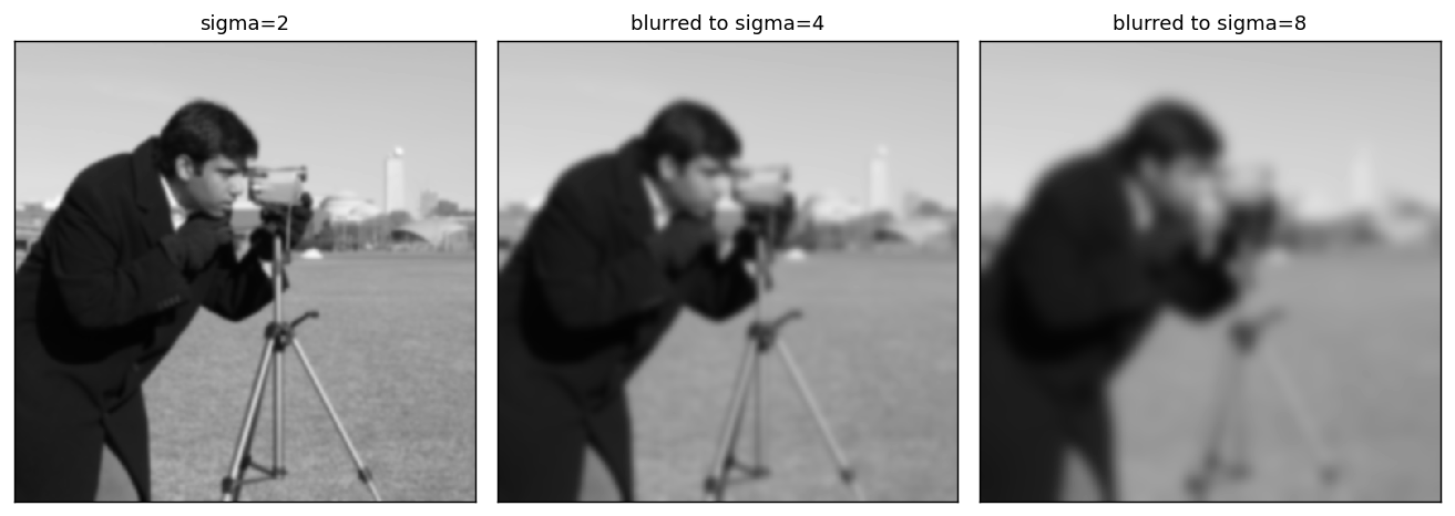 The book shows the same progression on a [photograph of a zebra](https://visionbook.mit.edu/blurring_2.html#fig-zebragaussian).
### Properties of the Gaussian
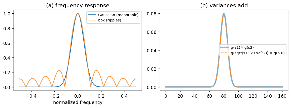
1. **Its Fourier transform is another Gaussian**, $G(\omega;\sigma)=e^{-\omega^2\sigma^2/2}$, which is **monotonically decreasing**, with no side lobes (contrast Figure 17.3b). A wider Gaussian in space is a *narrower* one in frequency.
2. **Composition adds variances:** $g(\sigma_1)*g(\sigma_2)=g(\sigma_3)$ with $\sigma_3^2=\sigma_1^2+\sigma_2^2$. Blurring twice is blurring once by a larger $\sigma$.
Both properties hold *exactly* only in the continuous case; the sampled kernel satisfies them to a close approximation.
```python theme={null}
# (left) monotonic Gaussian frequency response vs the rippled box;
# (right) numerical check that g(s1) * g(s2) == g(sqrt(s1^2+s2^2)).
g = gaussian_1d(3.0, radius=32).numpy()
box = (np.ones(9) / 9)
NFFT = 512; freq = np.fft.fftshift(np.fft.fftfreq(NFFT))
Hg = np.abs(np.fft.fftshift(np.fft.fft(g, NFFT)))
Hb = np.abs(np.fft.fftshift(np.fft.fft(box, NFFT)))
s1, s2 = 3.0, 4.0
lhs = np.convolve(gaussian_1d(s1, 40).numpy(), gaussian_1d(s2, 40).numpy())
s3 = np.sqrt(s1**2 + s2**2)
r = (len(lhs) - 1) // 2
rhs = gaussian_1d(s3, r).numpy()
```
The book shows the same progression on a [photograph of a zebra](https://visionbook.mit.edu/blurring_2.html#fig-zebragaussian).
### Properties of the Gaussian
1. **Its Fourier transform is another Gaussian**, $G(\omega;\sigma)=e^{-\omega^2\sigma^2/2}$, which is **monotonically decreasing**, with no side lobes (contrast Figure 17.3b). A wider Gaussian in space is a *narrower* one in frequency.
2. **Composition adds variances:** $g(\sigma_1)*g(\sigma_2)=g(\sigma_3)$ with $\sigma_3^2=\sigma_1^2+\sigma_2^2$. Blurring twice is blurring once by a larger $\sigma$.
Both properties hold *exactly* only in the continuous case; the sampled kernel satisfies them to a close approximation.
```python theme={null}
# (left) monotonic Gaussian frequency response vs the rippled box;
# (right) numerical check that g(s1) * g(s2) == g(sqrt(s1^2+s2^2)).
g = gaussian_1d(3.0, radius=32).numpy()
box = (np.ones(9) / 9)
NFFT = 512; freq = np.fft.fftshift(np.fft.fftfreq(NFFT))
Hg = np.abs(np.fft.fftshift(np.fft.fft(g, NFFT)))
Hb = np.abs(np.fft.fftshift(np.fft.fft(box, NFFT)))
s1, s2 = 3.0, 4.0
lhs = np.convolve(gaussian_1d(s1, 40).numpy(), gaussian_1d(s2, 40).numpy())
s3 = np.sqrt(s1**2 + s2**2)
r = (len(lhs) - 1) // 2
rhs = gaussian_1d(s3, r).numpy()
```
 ```python theme={null}
print('len(lhs), len(rhs):', len(lhs), len(rhs))
print('max |lhs - rhs| :', np.abs(lhs - rhs).max())
```
```output theme={null}
len(lhs), len(rhs): 161 161
max |lhs - rhs| : 2.2351742e-08
```
### Blur as a perceptual low-pass: the block portrait
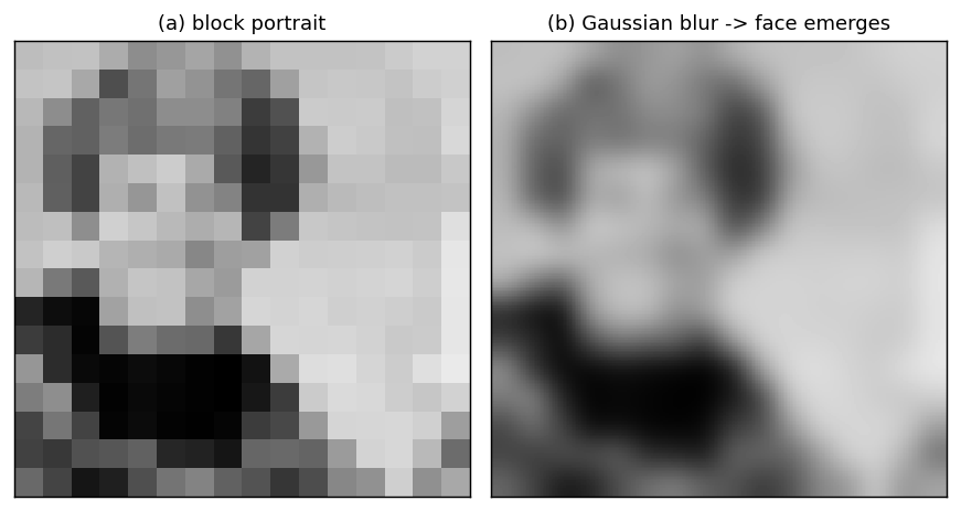
Harmon and Julesz's famous demonstration: a face quantized into coarse blocks is hard to read, because the **block edges inject high-frequency energy** that the visual system latches onto. Low-pass filtering (a Gaussian blur, or simply squinting) removes those spurious high frequencies and the face re-emerges. The book shows [the original block portrait of Lincoln](https://visionbook.mit.edu/blurring_2.html#fig-lincoln). Below you build a block portrait from a photograph by averaging it over $16\times16$ blocks, then blur it.
```python theme={null}
# Figure 17.5: a block portrait in the style of Harmon & Julesz (1971); blur reveals
# the face by removing the block-edge high frequencies.
# stand-in for Harmon and Julesz's block portrait of Lincoln in the book; original: https://visionbook.mit.edu/figures/blur_filters/Jules_Lincoln_1971.jpg
face = torch.from_numpy(rgb2gray(data.astronaut())[16:272, 136:392]).float() # 256 x 256 face crop
blocks = F.avg_pool2d(face[None, None], 16) # 16 x 16 block means
lincoln = F.interpolate(blocks, scale_factor=16, mode='nearest')[0, 0] # back to 256 x 256
revealed = conv2d(lincoln, gaussian_2d(8.0)) # sigma ~ half a block
```
```python theme={null}
print('len(lhs), len(rhs):', len(lhs), len(rhs))
print('max |lhs - rhs| :', np.abs(lhs - rhs).max())
```
```output theme={null}
len(lhs), len(rhs): 161 161
max |lhs - rhs| : 2.2351742e-08
```
### Blur as a perceptual low-pass: the block portrait
Harmon and Julesz's famous demonstration: a face quantized into coarse blocks is hard to read, because the **block edges inject high-frequency energy** that the visual system latches onto. Low-pass filtering (a Gaussian blur, or simply squinting) removes those spurious high frequencies and the face re-emerges. The book shows [the original block portrait of Lincoln](https://visionbook.mit.edu/blurring_2.html#fig-lincoln). Below you build a block portrait from a photograph by averaging it over $16\times16$ blocks, then blur it.
```python theme={null}
# Figure 17.5: a block portrait in the style of Harmon & Julesz (1971); blur reveals
# the face by removing the block-edge high frequencies.
# stand-in for Harmon and Julesz's block portrait of Lincoln in the book; original: https://visionbook.mit.edu/figures/blur_filters/Jules_Lincoln_1971.jpg
face = torch.from_numpy(rgb2gray(data.astronaut())[16:272, 136:392]).float() # 256 x 256 face crop
blocks = F.avg_pool2d(face[None, None], 16) # 16 x 16 block means
lincoln = F.interpolate(blocks, scale_factor=16, mode='nearest')[0, 0] # back to 256 x 256
revealed = conv2d(lincoln, gaussian_2d(8.0)) # sigma ~ half a block
```
 ## Binomial filters
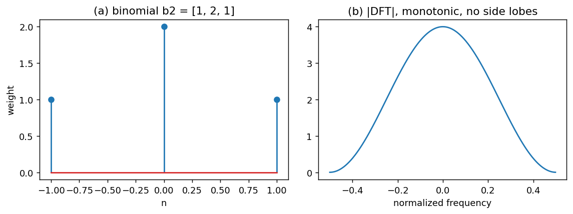
A **binomial filter** is what you get by convolving the elementary two-tap averager $[1,1]$ with itself $n$ times. The coefficients are the $n$-th row of **Pascal's triangle**:
$b_1=[1,1],\quad b_2=[1,2,1],\quad b_3=[1,3,3,1],\quad\dots$
Key facts (discrete analogues of the Gaussian's):
* **DC gain** $=\sum b_n = 2^n$, so normalize by $2^n$.
* **Variance** $\sigma_n^2 = n/4$.
* **Composition:** $b_n * b_m = b_{n+m}$ and $\sigma_n^2+\sigma_m^2=\sigma_{n+m}^2$.
* The Fourier magnitude $B_{2n}(u)=(2+2\cos(2\pi u/N))^n$ is **zero-phase and monotonic**: a discrete filter with no side lobes.
```python theme={null}
# Figure 17.7: the 1D binomial [1,2,1] and its monotonic Fourier magnitude.
def binomial_1d(n):
b = np.array([1.0])
for _ in range(n):
b = np.convolve(b, [1.0, 1.0]) # repeated [1,1] convolution
return b
b2 = binomial_1d(2) # [1, 2, 1]
var = np.sum(np.arange(-(len(b2)//2), len(b2)//2 + 1)**2 * b2) / b2.sum()
print('b2 :', b2, ' DC gain =', int(b2.sum()), '= 2^2')
print('variance :', var, ' (expected n/4 = 0.5)')
NFFT = 512; freq = np.fft.fftshift(np.fft.fftfreq(NFFT))
Hb2 = np.abs(np.fft.fftshift(np.fft.fft(b2, NFFT)))
```
```output theme={null}
b2 : [1. 2. 1.] DC gain = 4 = 2^2
variance : 0.5 (expected n/4 = 0.5)
```
## Binomial filters
A **binomial filter** is what you get by convolving the elementary two-tap averager $[1,1]$ with itself $n$ times. The coefficients are the $n$-th row of **Pascal's triangle**:
$b_1=[1,1],\quad b_2=[1,2,1],\quad b_3=[1,3,3,1],\quad\dots$
Key facts (discrete analogues of the Gaussian's):
* **DC gain** $=\sum b_n = 2^n$, so normalize by $2^n$.
* **Variance** $\sigma_n^2 = n/4$.
* **Composition:** $b_n * b_m = b_{n+m}$ and $\sigma_n^2+\sigma_m^2=\sigma_{n+m}^2$.
* The Fourier magnitude $B_{2n}(u)=(2+2\cos(2\pi u/N))^n$ is **zero-phase and monotonic**: a discrete filter with no side lobes.
```python theme={null}
# Figure 17.7: the 1D binomial [1,2,1] and its monotonic Fourier magnitude.
def binomial_1d(n):
b = np.array([1.0])
for _ in range(n):
b = np.convolve(b, [1.0, 1.0]) # repeated [1,1] convolution
return b
b2 = binomial_1d(2) # [1, 2, 1]
var = np.sum(np.arange(-(len(b2)//2), len(b2)//2 + 1)**2 * b2) / b2.sum()
print('b2 :', b2, ' DC gain =', int(b2.sum()), '= 2^2')
print('variance :', var, ' (expected n/4 = 0.5)')
NFFT = 512; freq = np.fft.fftshift(np.fft.fftfreq(NFFT))
Hb2 = np.abs(np.fft.fftshift(np.fft.fft(b2, NFFT)))
```
```output theme={null}
b2 : [1. 2. 1.] DC gain = 4 = 2^2
variance : 0.5 (expected n/4 = 0.5)
```
 ### 2D binomial filters and perfect cancellation of the checkerboard
By separability the 2D binomial is the outer product $b_{2,2}=[1,2,1]^\top[1,2,1]$, i.e.
$\tfrac{1}{16}\begin{bmatrix}1&2&1\\2&4&2\\1&2&1\end{bmatrix}.$
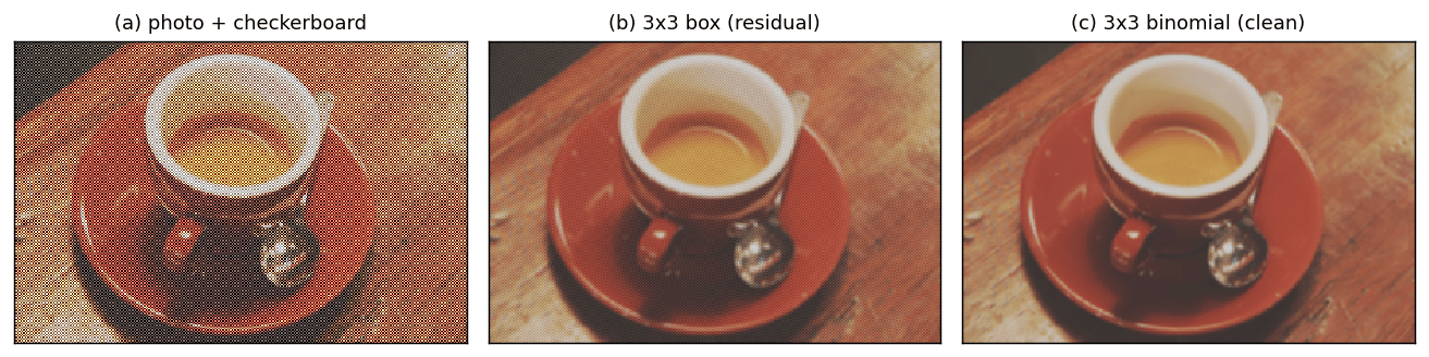
The highest representable frequency is the alternating wave $[\dots,1,-1,1,-1,\dots]$. Convolving it with $[1,2,1]/4$ gives $(1-2+1)/4 = 0$, so the binomial **annihilates the checkerboard exactly**. The box $[1,1,1]/3$ leaves a residual $(1-1+1)/3 = 1/3$. Figure 17.8 shows this on an image corrupted by a checkerboard pattern. The book uses a [photograph of a boat](https://visionbook.mit.edu/blurring_2.html#fig-boat_b_noise).
```python theme={null}
# Figure 17.8: checkerboard cancellation on a color photo.
# The book displays the checkerboard as 8x8-pixel squares (an 8x upscaled view);
# on the actual sampling grid it is the 1-pixel Nyquist wave [1,-1,...]. Take a
# color photo, add that 1-pixel checkerboard, then filter: the 3x3 box leaves
# a 1/3 residual, while the 3x3 binomial [1,2,1]^2/16 annihilates it exactly.
# stand-in for a photograph of a boat in the book; original: https://visionbook.mit.edu/figures/blur_filters/boat_d_binomial.jpg
boat = clean # the clean color photo from Figure 17.1
Hb, Wb = boat.shape[:2]
yy, xx = torch.meshgrid(torch.arange(Hb), torch.arange(Wb), indexing='ij')
checker = ((xx + yy) % 2 == 0).float() * 2 - 1 # +-1 alternating (highest freq)
corrupt = (boat + 0.4 * checker[..., None]).clamp(0, 1) # same checker added to R, G, B
box3 = torch.ones(3, 3) / 9.0
b = torch.tensor(binomial_1d(2), dtype=torch.float32)
bin2d = torch.outer(b, b); bin2d = bin2d / bin2d.sum() # [1,2,1]^2 / 16
out_box = conv2d_rgb(corrupt, box3)
out_bin = conv2d_rgb(corrupt, bin2d)
```
### 2D binomial filters and perfect cancellation of the checkerboard
By separability the 2D binomial is the outer product $b_{2,2}=[1,2,1]^\top[1,2,1]$, i.e.
$\tfrac{1}{16}\begin{bmatrix}1&2&1\\2&4&2\\1&2&1\end{bmatrix}.$
The highest representable frequency is the alternating wave $[\dots,1,-1,1,-1,\dots]$. Convolving it with $[1,2,1]/4$ gives $(1-2+1)/4 = 0$, so the binomial **annihilates the checkerboard exactly**. The box $[1,1,1]/3$ leaves a residual $(1-1+1)/3 = 1/3$. Figure 17.8 shows this on an image corrupted by a checkerboard pattern. The book uses a [photograph of a boat](https://visionbook.mit.edu/blurring_2.html#fig-boat_b_noise).
```python theme={null}
# Figure 17.8: checkerboard cancellation on a color photo.
# The book displays the checkerboard as 8x8-pixel squares (an 8x upscaled view);
# on the actual sampling grid it is the 1-pixel Nyquist wave [1,-1,...]. Take a
# color photo, add that 1-pixel checkerboard, then filter: the 3x3 box leaves
# a 1/3 residual, while the 3x3 binomial [1,2,1]^2/16 annihilates it exactly.
# stand-in for a photograph of a boat in the book; original: https://visionbook.mit.edu/figures/blur_filters/boat_d_binomial.jpg
boat = clean # the clean color photo from Figure 17.1
Hb, Wb = boat.shape[:2]
yy, xx = torch.meshgrid(torch.arange(Hb), torch.arange(Wb), indexing='ij')
checker = ((xx + yy) % 2 == 0).float() * 2 - 1 # +-1 alternating (highest freq)
corrupt = (boat + 0.4 * checker[..., None]).clamp(0, 1) # same checker added to R, G, B
box3 = torch.ones(3, 3) / 9.0
b = torch.tensor(binomial_1d(2), dtype=torch.float32)
bin2d = torch.outer(b, b); bin2d = bin2d / bin2d.sum() # [1,2,1]^2 / 16
out_box = conv2d_rgb(corrupt, box3)
out_bin = conv2d_rgb(corrupt, bin2d)
```
 ```python theme={null}
print('recovered-vs-clean error, box :', (out_box - boat).abs().mean().item())
print('recovered-vs-clean error, binomial:', (out_bin - boat).abs().mean().item())
print('residual checkerboard , binomial:', (out_bin * checker[..., None]).mean().abs().item())
```
```output theme={null}
recovered-vs-clean error, box : 0.10610868036746979
recovered-vs-clean error, binomial: 0.09788819402456284
residual checkerboard , binomial: 2.32934962696163e-06
```
### Binomials converge to the Gaussian
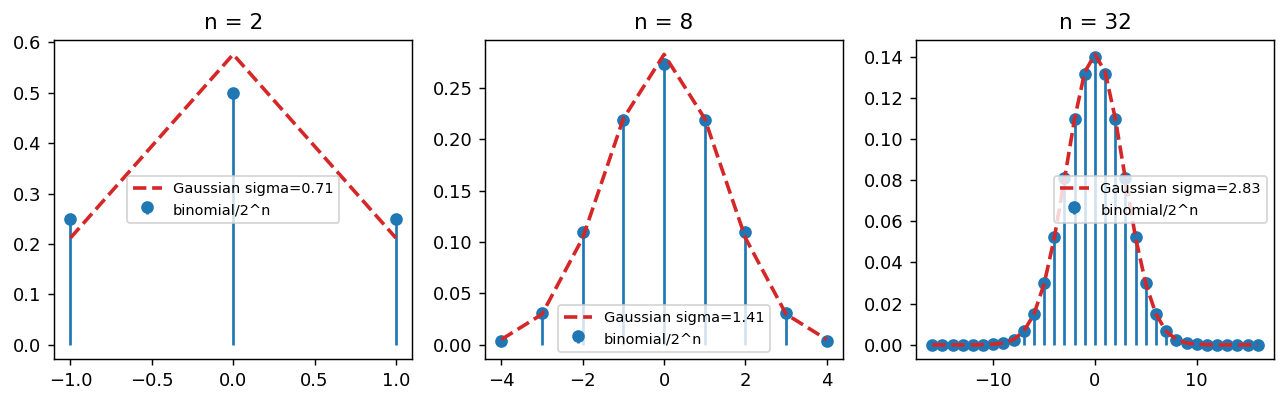
Repeatedly convolving $[1,1]$ is repeated averaging, so by the **central limit theorem** the normalized binomial $b_n/2^n$ approaches a Gaussian of variance $n/4$ as $n$ grows. This is why small binomials (e.g. $[1,2,1]$, $[1,4,6,4,1]$) are the standard cheap, integer-arithmetic Gaussian approximations used in image pyramids.
```python theme={null}
# Overlay the normalized binomial b_n against the Gaussian of matching variance.
```
```python theme={null}
print('recovered-vs-clean error, box :', (out_box - boat).abs().mean().item())
print('recovered-vs-clean error, binomial:', (out_bin - boat).abs().mean().item())
print('residual checkerboard , binomial:', (out_bin * checker[..., None]).mean().abs().item())
```
```output theme={null}
recovered-vs-clean error, box : 0.10610868036746979
recovered-vs-clean error, binomial: 0.09788819402456284
residual checkerboard , binomial: 2.32934962696163e-06
```
### Binomials converge to the Gaussian
Repeatedly convolving $[1,1]$ is repeated averaging, so by the **central limit theorem** the normalized binomial $b_n/2^n$ approaches a Gaussian of variance $n/4$ as $n$ grows. This is why small binomials (e.g. $[1,2,1]$, $[1,4,6,4,1]$) are the standard cheap, integer-arithmetic Gaussian approximations used in image pyramids.
```python theme={null}
# Overlay the normalized binomial b_n against the Gaussian of matching variance.
```
 ## Concluding remarks
Three blur filters, one theme, a **low-pass average**:
| Filter | Kernel | Frequency response | Notes |
| - | - | - | - |
| **Box** | uniform window | sinc: **side lobes** | cheapest; separable; artifacts |
| **Gaussian** | $e^{-x^2/2\sigma^2}$ | Gaussian: **monotonic** | isotropic; only separable circular kernel; variances add |
| **Binomial** | Pascal's row $/2^n$ | $(2+2\cos)^n$: **monotonic** | integer Gaussian approx; $b_n*b_m=b_{n+m}$; cancels the checkerboard |
The box is fast but its ripples pass spurious high frequencies. The Gaussian is the ideal isotropic low-pass and composes cleanly under $\sigma^2$ addition. The binomial is the practical, integer-arithmetic bridge, a discrete filter that keeps the Gaussian's good behavior and, by the central limit theorem, *becomes* a Gaussian in the limit. These are the building blocks for **downsampling, upsampling, and image pyramids** in the chapters that follow.
***
[Edit this page on GitHub](https://github.com/aegean-ai/eaia/edit/main/src/aiml-common/lectures/image-processing/blur-filters/index.mdx) or [file an issue](https://github.com/aegean-ai/eaia/issues/new/choose).
## Concluding remarks
Three blur filters, one theme, a **low-pass average**:
| Filter | Kernel | Frequency response | Notes |
| - | - | - | - |
| **Box** | uniform window | sinc: **side lobes** | cheapest; separable; artifacts |
| **Gaussian** | $e^{-x^2/2\sigma^2}$ | Gaussian: **monotonic** | isotropic; only separable circular kernel; variances add |
| **Binomial** | Pascal's row $/2^n$ | $(2+2\cos)^n$: **monotonic** | integer Gaussian approx; $b_n*b_m=b_{n+m}$; cancels the checkerboard |
The box is fast but its ripples pass spurious high frequencies. The Gaussian is the ideal isotropic low-pass and composes cleanly under $\sigma^2$ addition. The binomial is the practical, integer-arithmetic bridge, a discrete filter that keeps the Gaussian's good behavior and, by the central limit theorem, *becomes* a Gaussian in the limit. These are the building blocks for **downsampling, upsampling, and image pyramids** in the chapters that follow.
***
[Edit this page on GitHub](https://github.com/aegean-ai/eaia/edit/main/src/aiml-common/lectures/image-processing/blur-filters/index.mdx) or [file an issue](https://github.com/aegean-ai/eaia/issues/new/choose).