> ## Documentation Index
> Fetch the complete documentation index at: https://aegean.ai/llms.txt
> Use this file to discover all available pages before exploring further.
# Measuring Change with Image Derivatives
> Discrete and Gaussian derivatives, the Laplacian, edge operators, unsharp masking, and Retinex.
 *This section was written by [Kaushik Kachireddy](https://github.com/kaushik0x7d2) ([pull request #77](https://github.com/pantelis/eng-ai-agents/pull/77)), with help from an AI coding agent (Claude Code) on the code. It reproduces the ideas of Chapter 18 of [*Foundations of Computer Vision*](https://visionbook.mit.edu/derivatives.html) by Antonio Torralba, Phillip Isola, and William T. Freeman. The book's own figures are not reproduced here, because the book's license covers only the work in full; links point to them instead.*
The image derivative is the workhorse of low-level vision: it turns intensity changes into signals you can measure. This section builds the derivative operators of the book's chapter: the two-tap $[1,-1]$ and centered $[1,0,-1]$ kernels, **Gaussian derivatives** (through Hermite polynomials), **derivative-of-binomial** kernels, the **Roberts and Sobel** operators, the **Laplacian** and Laplacian-of-Gaussian, **unsharp masking**, and a working **Retinex** decomposition. Each comes with a numerical check.
The book demonstrates these operators on its own photographs. Here they run on scikit-image test images and on synthetic patterns, with a link to each of the book's figures. Following the book, derivative maps are shown **signed around mid-gray**, per channel, so color inputs show colored edges.
```python theme={null}
import numpy as np
import torch
import torch.nn.functional as F
import matplotlib.pyplot as plt
from numpy.polynomial.hermite import hermval
from skimage import data, img_as_float
_ = torch.manual_seed(0); np.random.seed(0)
torch.set_default_dtype(torch.float32)
plt.rcParams.update({'figure.dpi': 130, 'savefig.dpi': 130,
'image.cmap': 'gray', 'image.interpolation': 'nearest', 'axes.grid': False})
```
**Images replaced for licensing.** The book is published under a CC BY-NC-ND license, which covers only the book as a whole and not its individual images, so this page does not republish the book's photographs. License-free images stand in for them:
* The *astronaut* photograph (scikit-image) stands in for [a color photograph of the MIT dome (Figure 18.2)](https://visionbook.mit.edu/figures/derivatives/mit_der_a.jpg).
* The *coffee* photograph with added noise (scikit-image) stands in for [a noisy photograph of a stop sign (Figure 18.6)](https://visionbook.mit.edu/figures/derivatives/stop_noise.jpg).
* The *cameraman* photograph (scikit-image) stands in for [a photograph of a zebra (Figure 18.8)](https://visionbook.mit.edu/derivatives.html#fig-gaussiander_zebra).
* A generated spoked wheel stands in for [a photograph of a wheel (Figure 18.18)](https://visionbook.mit.edu/figures/spatial_filters/wheel256.jpg).
* The *coffee* photograph (scikit-image) stands in for [a photograph of a boat (Figure 18.23)](https://visionbook.mit.edu/figures/spatial_filters/boat_sharp0.jpg).
If you use the book for non-commercial purposes, you can swap the originals back in: each line that loads a stand-in carries the original's link in a comment.
```python theme={null}
def conv2d(image, kernel, mode='reflect'):
"""2D convolution, "same" size, reflect-padded (kernels here are symmetric-ish)."""
k = torch.as_tensor(kernel, dtype=torch.float32).flip(0).flip(1)
kh, kw = k.shape
x = F.pad(image[None, None], (kw // 2, kw // 2, kh // 2, kh // 2), mode=mode)
return F.conv2d(x, k[None, None])[0, 0]
def conv2d_rgb(image, kernel, mode='reflect'):
return torch.stack([conv2d(image[..., c], kernel, mode) for c in range(3)], dim=-1)
def gaussian_1d(sigma, radius=None):
if radius is None:
radius = int(np.ceil(3 * sigma))
x = torch.arange(-radius, radius + 1, dtype=torch.float32)
k = torch.exp(-x**2 / (2 * sigma**2))
return k / k.sum()
def dgauss_1d(sigma, order, radius=None):
"""n-th derivative of a unit-area 1D Gaussian, via Hermite polynomials:
g_{x^n}(x) = (-1/(sigma*sqrt2))^n H_n(x/(sigma*sqrt2)) g(x).
"""
if radius is None:
radius = int(np.ceil(4 * sigma)) + order
x = np.arange(-radius, radius + 1, dtype=np.float64)
g = np.exp(-x**2 / (2 * sigma**2)) / (sigma * np.sqrt(2 * np.pi))
a = x / (sigma * np.sqrt(2))
Hn = hermval(a, [0] * order + [1])
k = ((-1.0 / (sigma * np.sqrt(2))) ** order) * Hn * g
return torch.tensor(k, dtype=torch.float32)
def gauss_deriv2d(sigma, nx, ny):
"""Separable 2D Gaussian derivative kernel (order nx in x, ny in y)."""
kx = dgauss_1d(sigma, nx); ky = dgauss_1d(sigma, ny)
return torch.outer(ky, kx)
def grad_mag(image, kx, ky):
return torch.sqrt(conv2d(image, kx)**2 + conv2d(image, ky)**2 + 1e-12)
```
```python theme={null}
def luminance(rgb):
w = torch.tensor([0.299, 0.587, 0.114])
return (rgb * w).sum(-1)
# Standard finite-difference kernels used throughout.
D0 = torch.tensor([[1.0, -1.0]]) # two-tap [1, -1]
D1 = torch.tensor([[1.0, 0.0, -1.0]]) / 2.0 # centered [1, 0, -1] / 2
```
```python theme={null}
# Test images: a color photo (astronaut), a grayscale photo (cameraman), and a
# color photo at 300 x 200 (coffee), all float32 in [0, 1].
def as_tensor(img):
return torch.from_numpy(img_as_float(img)).float()
photo_rgb = F.avg_pool2d(as_tensor(data.astronaut()).permute(2, 0, 1)[None], 2)[0].permute(1, 2, 0) # 256 x 256
coffee_rgb = F.avg_pool2d(as_tensor(data.coffee()).permute(2, 0, 1)[None], 2)[0].permute(1, 2, 0) # 200 x 300
camera = as_tensor(data.camera()) # 512 x 512
```
## Discretizing the image derivative
The continuous partial derivative $\partial\ell/\partial x$ becomes a finite difference. Two choices dominate:
$d_0 = [1,\,-1]\ (\ell[n]-\ell[n-1]),\qquad d_1 = \tfrac12[1,\,0,\,-1]\ \bigl(\tfrac{\ell[n+1]-\ell[n-1]}{2}\bigr).$
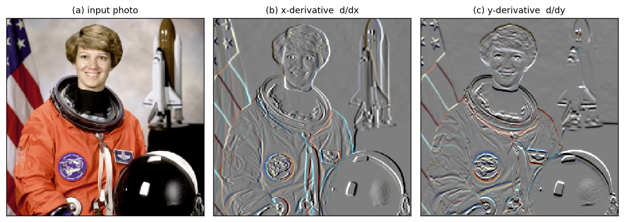
$d_0$ is a half-pixel-shifted difference; $d_1$ is **centered** (no shift) and a touch smoother. Applying $d_1$ across $x$ and down $y$ gives the two derivative images of Figure 18.2 ([the book's version](https://visionbook.mit.edu/derivatives.html#fig-derivativesmit)). Following the book, the derivative of each color channel is shown **signed around mid-gray**: light where intensity rises and dark where it falls, which paints edges in blue/orange.
```python theme={null}
# Figure 18.2: x/y derivatives of a color photo, shown the book's way:
# the SIGNED derivative of each color channel around mid-gray (blue/orange edges).
# stand-in for a color photograph of the MIT dome in the book; original: https://visionbook.mit.edu/figures/derivatives/mit_der_a.jpg
photo = photo_rgb
dx = conv2d_rgb(photo, D1)
dy = conv2d_rgb(photo, D1.T)
```
*This section was written by [Kaushik Kachireddy](https://github.com/kaushik0x7d2) ([pull request #77](https://github.com/pantelis/eng-ai-agents/pull/77)), with help from an AI coding agent (Claude Code) on the code. It reproduces the ideas of Chapter 18 of [*Foundations of Computer Vision*](https://visionbook.mit.edu/derivatives.html) by Antonio Torralba, Phillip Isola, and William T. Freeman. The book's own figures are not reproduced here, because the book's license covers only the work in full; links point to them instead.*
The image derivative is the workhorse of low-level vision: it turns intensity changes into signals you can measure. This section builds the derivative operators of the book's chapter: the two-tap $[1,-1]$ and centered $[1,0,-1]$ kernels, **Gaussian derivatives** (through Hermite polynomials), **derivative-of-binomial** kernels, the **Roberts and Sobel** operators, the **Laplacian** and Laplacian-of-Gaussian, **unsharp masking**, and a working **Retinex** decomposition. Each comes with a numerical check.
The book demonstrates these operators on its own photographs. Here they run on scikit-image test images and on synthetic patterns, with a link to each of the book's figures. Following the book, derivative maps are shown **signed around mid-gray**, per channel, so color inputs show colored edges.
```python theme={null}
import numpy as np
import torch
import torch.nn.functional as F
import matplotlib.pyplot as plt
from numpy.polynomial.hermite import hermval
from skimage import data, img_as_float
_ = torch.manual_seed(0); np.random.seed(0)
torch.set_default_dtype(torch.float32)
plt.rcParams.update({'figure.dpi': 130, 'savefig.dpi': 130,
'image.cmap': 'gray', 'image.interpolation': 'nearest', 'axes.grid': False})
```
**Images replaced for licensing.** The book is published under a CC BY-NC-ND license, which covers only the book as a whole and not its individual images, so this page does not republish the book's photographs. License-free images stand in for them:
* The *astronaut* photograph (scikit-image) stands in for [a color photograph of the MIT dome (Figure 18.2)](https://visionbook.mit.edu/figures/derivatives/mit_der_a.jpg).
* The *coffee* photograph with added noise (scikit-image) stands in for [a noisy photograph of a stop sign (Figure 18.6)](https://visionbook.mit.edu/figures/derivatives/stop_noise.jpg).
* The *cameraman* photograph (scikit-image) stands in for [a photograph of a zebra (Figure 18.8)](https://visionbook.mit.edu/derivatives.html#fig-gaussiander_zebra).
* A generated spoked wheel stands in for [a photograph of a wheel (Figure 18.18)](https://visionbook.mit.edu/figures/spatial_filters/wheel256.jpg).
* The *coffee* photograph (scikit-image) stands in for [a photograph of a boat (Figure 18.23)](https://visionbook.mit.edu/figures/spatial_filters/boat_sharp0.jpg).
If you use the book for non-commercial purposes, you can swap the originals back in: each line that loads a stand-in carries the original's link in a comment.
```python theme={null}
def conv2d(image, kernel, mode='reflect'):
"""2D convolution, "same" size, reflect-padded (kernels here are symmetric-ish)."""
k = torch.as_tensor(kernel, dtype=torch.float32).flip(0).flip(1)
kh, kw = k.shape
x = F.pad(image[None, None], (kw // 2, kw // 2, kh // 2, kh // 2), mode=mode)
return F.conv2d(x, k[None, None])[0, 0]
def conv2d_rgb(image, kernel, mode='reflect'):
return torch.stack([conv2d(image[..., c], kernel, mode) for c in range(3)], dim=-1)
def gaussian_1d(sigma, radius=None):
if radius is None:
radius = int(np.ceil(3 * sigma))
x = torch.arange(-radius, radius + 1, dtype=torch.float32)
k = torch.exp(-x**2 / (2 * sigma**2))
return k / k.sum()
def dgauss_1d(sigma, order, radius=None):
"""n-th derivative of a unit-area 1D Gaussian, via Hermite polynomials:
g_{x^n}(x) = (-1/(sigma*sqrt2))^n H_n(x/(sigma*sqrt2)) g(x).
"""
if radius is None:
radius = int(np.ceil(4 * sigma)) + order
x = np.arange(-radius, radius + 1, dtype=np.float64)
g = np.exp(-x**2 / (2 * sigma**2)) / (sigma * np.sqrt(2 * np.pi))
a = x / (sigma * np.sqrt(2))
Hn = hermval(a, [0] * order + [1])
k = ((-1.0 / (sigma * np.sqrt(2))) ** order) * Hn * g
return torch.tensor(k, dtype=torch.float32)
def gauss_deriv2d(sigma, nx, ny):
"""Separable 2D Gaussian derivative kernel (order nx in x, ny in y)."""
kx = dgauss_1d(sigma, nx); ky = dgauss_1d(sigma, ny)
return torch.outer(ky, kx)
def grad_mag(image, kx, ky):
return torch.sqrt(conv2d(image, kx)**2 + conv2d(image, ky)**2 + 1e-12)
```
```python theme={null}
def luminance(rgb):
w = torch.tensor([0.299, 0.587, 0.114])
return (rgb * w).sum(-1)
# Standard finite-difference kernels used throughout.
D0 = torch.tensor([[1.0, -1.0]]) # two-tap [1, -1]
D1 = torch.tensor([[1.0, 0.0, -1.0]]) / 2.0 # centered [1, 0, -1] / 2
```
```python theme={null}
# Test images: a color photo (astronaut), a grayscale photo (cameraman), and a
# color photo at 300 x 200 (coffee), all float32 in [0, 1].
def as_tensor(img):
return torch.from_numpy(img_as_float(img)).float()
photo_rgb = F.avg_pool2d(as_tensor(data.astronaut()).permute(2, 0, 1)[None], 2)[0].permute(1, 2, 0) # 256 x 256
coffee_rgb = F.avg_pool2d(as_tensor(data.coffee()).permute(2, 0, 1)[None], 2)[0].permute(1, 2, 0) # 200 x 300
camera = as_tensor(data.camera()) # 512 x 512
```
## Discretizing the image derivative
The continuous partial derivative $\partial\ell/\partial x$ becomes a finite difference. Two choices dominate:
$d_0 = [1,\,-1]\ (\ell[n]-\ell[n-1]),\qquad d_1 = \tfrac12[1,\,0,\,-1]\ \bigl(\tfrac{\ell[n+1]-\ell[n-1]}{2}\bigr).$
$d_0$ is a half-pixel-shifted difference; $d_1$ is **centered** (no shift) and a touch smoother. Applying $d_1$ across $x$ and down $y$ gives the two derivative images of Figure 18.2 ([the book's version](https://visionbook.mit.edu/derivatives.html#fig-derivativesmit)). Following the book, the derivative of each color channel is shown **signed around mid-gray**: light where intensity rises and dark where it falls, which paints edges in blue/orange.
```python theme={null}
# Figure 18.2: x/y derivatives of a color photo, shown the book's way:
# the SIGNED derivative of each color channel around mid-gray (blue/orange edges).
# stand-in for a color photograph of the MIT dome in the book; original: https://visionbook.mit.edu/figures/derivatives/mit_der_a.jpg
photo = photo_rgb
dx = conv2d_rgb(photo, D1)
dy = conv2d_rgb(photo, D1.T)
```
 ```python theme={null}
print('mean |d/dx|:', dx.abs().mean().item(), ' mean |d/dy|:', dy.abs().mean().item())
```
```output theme={null}
mean |d/dx|: 0.03433092311024666 mean |d/dy|: 0.027904972434043884
```
### What the two kernels do in frequency
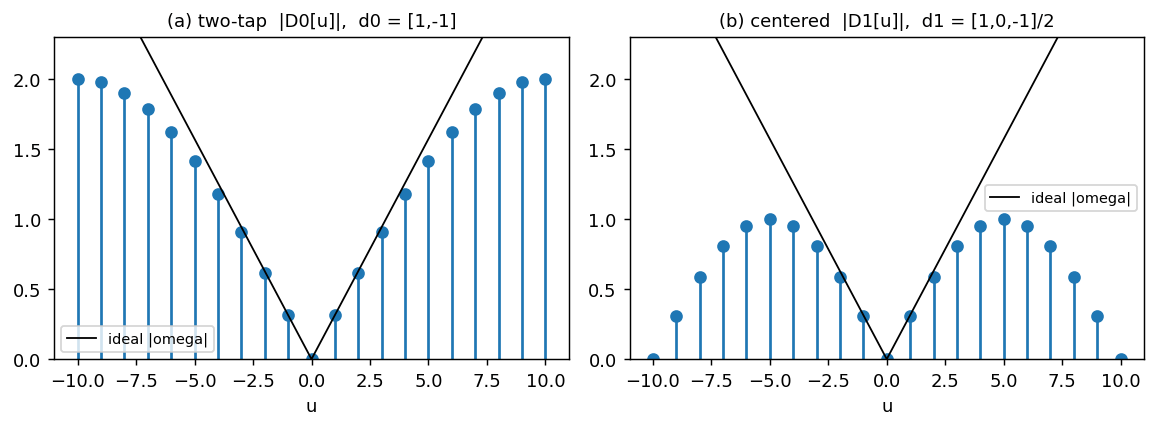
An ideal derivative multiplies each frequency by $j\omega$, i.e. magnitude grows **linearly** with frequency. The DFTs
$D_0[u] = 1-e^{-2\pi j u/N},\ |D_0| = 2\sin(\pi u/N),\qquad D_1[u] = j\sin(2\pi u/N),$
both approximate $|\omega|$ at low frequencies. $|D_0|$ tracks the ideal further up the band; $|D_1|$ rolls off earlier (it suppresses the highest frequencies, so it is smoother and less noisy).
```python theme={null}
# Figure 18.4: |DFT| of d0 and d1 vs the ideal |omega|, as discrete stems over
# u = -N/2 .. N/2 (as the book draws them), with the ideal shown as a line.
N = 20
u = np.arange(-N // 2, N // 2 + 1) # -10 .. 10
ideal = np.abs(2 * np.pi * u / N) # ideal derivative response |omega|
D0m = np.abs(1 - np.exp(-2j * np.pi * u / N)) # = 2 sin(pi u / N)
D1m = np.abs(np.sin(2 * np.pi * u / N))
```
```python theme={null}
print('mean |d/dx|:', dx.abs().mean().item(), ' mean |d/dy|:', dy.abs().mean().item())
```
```output theme={null}
mean |d/dx|: 0.03433092311024666 mean |d/dy|: 0.027904972434043884
```
### What the two kernels do in frequency
An ideal derivative multiplies each frequency by $j\omega$, i.e. magnitude grows **linearly** with frequency. The DFTs
$D_0[u] = 1-e^{-2\pi j u/N},\ |D_0| = 2\sin(\pi u/N),\qquad D_1[u] = j\sin(2\pi u/N),$
both approximate $|\omega|$ at low frequencies. $|D_0|$ tracks the ideal further up the band; $|D_1|$ rolls off earlier (it suppresses the highest frequencies, so it is smoother and less noisy).
```python theme={null}
# Figure 18.4: |DFT| of d0 and d1 vs the ideal |omega|, as discrete stems over
# u = -N/2 .. N/2 (as the book draws them), with the ideal shown as a line.
N = 20
u = np.arange(-N // 2, N // 2 + 1) # -10 .. 10
ideal = np.abs(2 * np.pi * u / N) # ideal derivative response |omega|
D0m = np.abs(1 - np.exp(-2j * np.pi * u / N)) # = 2 sin(pi u / N)
D1m = np.abs(np.sin(2 * np.pi * u / N))
```
 ## Gaussian derivatives beat noise
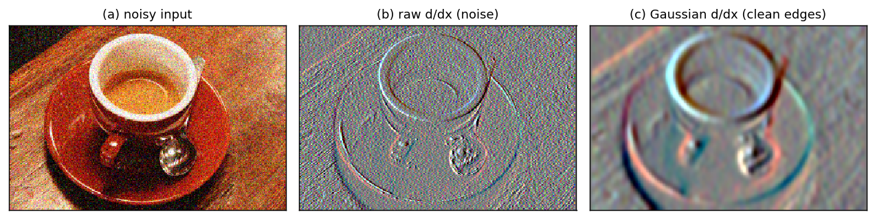
Differentiation amplifies high frequencies, so a raw $[1,-1]$ derivative of a noisy image is dominated by noise. Because differentiation and convolution commute,
$\frac{\partial \ell}{\partial x}*g = \ell * \frac{\partial g}{\partial x},$
you can differentiate the **smooth Gaussian** instead of the noisy image. The first Gaussian derivative $g_x=-\tfrac{x}{\sigma^2}g$ smooths and differentiates in one pass. Figure 18.6 contrasts the two on a noisy photo ([the book's version](https://visionbook.mit.edu/derivatives.html#fig-derivativesnoisystop)).
```python theme={null}
# Figure 18.6: raw x-derivative (noise-amplified) vs Gaussian x-derivative.
# Shown the way the book does it: the SIGNED derivative of each color channel,
# displayed around mid-gray (light = positive edge, dark = negative edge).
# stand-in for a noisy photograph of a stop sign in the book; original: https://visionbook.mit.edu/figures/derivatives/stop_noise.jpg
noisy = (coffee_rgb + 0.12 * torch.randn_like(coffee_rgb)).clamp(0, 1) # additive Gaussian noise
raw = conv2d_rgb(noisy, D1) # raw centered difference, per channel
gauss = conv2d_rgb(noisy, gauss_deriv2d(3.0, 1, 0)) # Gaussian x-derivative, sigma=3
```
## Gaussian derivatives beat noise
Differentiation amplifies high frequencies, so a raw $[1,-1]$ derivative of a noisy image is dominated by noise. Because differentiation and convolution commute,
$\frac{\partial \ell}{\partial x}*g = \ell * \frac{\partial g}{\partial x},$
you can differentiate the **smooth Gaussian** instead of the noisy image. The first Gaussian derivative $g_x=-\tfrac{x}{\sigma^2}g$ smooths and differentiates in one pass. Figure 18.6 contrasts the two on a noisy photo ([the book's version](https://visionbook.mit.edu/derivatives.html#fig-derivativesnoisystop)).
```python theme={null}
# Figure 18.6: raw x-derivative (noise-amplified) vs Gaussian x-derivative.
# Shown the way the book does it: the SIGNED derivative of each color channel,
# displayed around mid-gray (light = positive edge, dark = negative edge).
# stand-in for a noisy photograph of a stop sign in the book; original: https://visionbook.mit.edu/figures/derivatives/stop_noise.jpg
noisy = (coffee_rgb + 0.12 * torch.randn_like(coffee_rgb)).clamp(0, 1) # additive Gaussian noise
raw = conv2d_rgb(noisy, D1) # raw centered difference, per channel
gauss = conv2d_rgb(noisy, gauss_deriv2d(3.0, 1, 0)) # Gaussian x-derivative, sigma=3
```
 ```python theme={null}
print('background derivative std, raw :', raw[:80, :80].std().item())
print('background derivative std, gauss :', gauss[:80, :80].std().item(),
' # Gaussian derivative suppresses the noise floor')
```
```output theme={null}
background derivative std, raw : 0.08325188606977463
background derivative std, gauss : 0.008138191886246204 # Gaussian derivative suppresses the noise floor
```
## Gaussian derivatives and the Hermite family
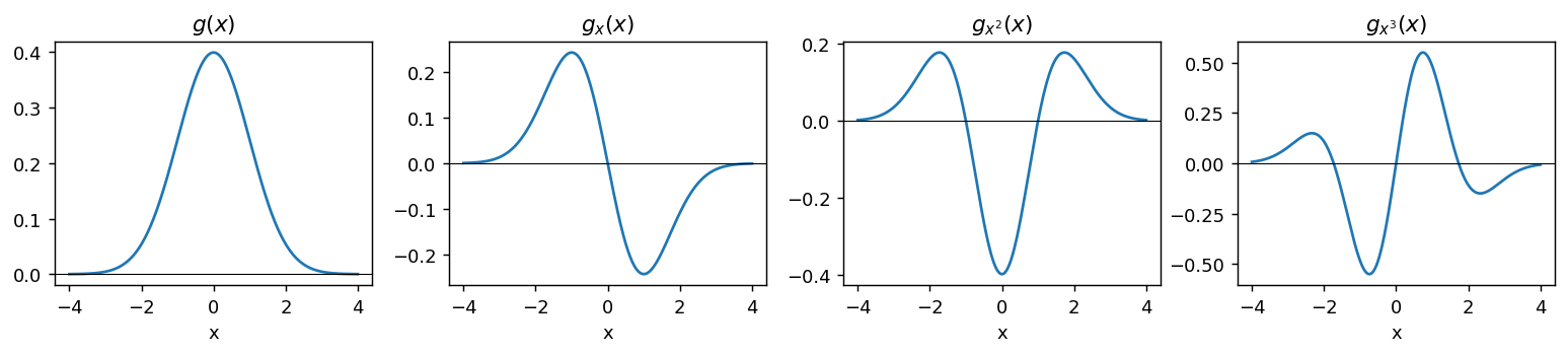
Higher derivative orders of the Gaussian are Hermite polynomials times the Gaussian:
$g_{x^n}(x;\sigma) = \Bigl(\tfrac{-1}{\sigma\sqrt2}\Bigr)^n H_n\!\Bigl(\tfrac{x}{\sigma\sqrt2}\Bigr)\,g(x;\sigma),\qquad H_n(x)=2xH_{n-1}-2(n-1)H_{n-2}.$
Each order adds one more oscillation. Orders 0 to 3 for $\sigma=1$:
```python theme={null}
# Figure 18.9: the Gaussian and its first three derivatives, sigma = 1
# (smooth continuous curves over x in [-4, 4], as in the book).
x = np.linspace(-4, 4, 400)
g = np.exp(-x**2 / 2) / np.sqrt(2 * np.pi)
a = x / np.sqrt(2)
titles = ['$g(x)$', '$g_x(x)$', '$g_{x^2}(x)$', '$g_{x^3}(x)$']
```
```python theme={null}
print('background derivative std, raw :', raw[:80, :80].std().item())
print('background derivative std, gauss :', gauss[:80, :80].std().item(),
' # Gaussian derivative suppresses the noise floor')
```
```output theme={null}
background derivative std, raw : 0.08325188606977463
background derivative std, gauss : 0.008138191886246204 # Gaussian derivative suppresses the noise floor
```
## Gaussian derivatives and the Hermite family
Higher derivative orders of the Gaussian are Hermite polynomials times the Gaussian:
$g_{x^n}(x;\sigma) = \Bigl(\tfrac{-1}{\sigma\sqrt2}\Bigr)^n H_n\!\Bigl(\tfrac{x}{\sigma\sqrt2}\Bigr)\,g(x;\sigma),\qquad H_n(x)=2xH_{n-1}-2(n-1)H_{n-2}.$
Each order adds one more oscillation. Orders 0 to 3 for $\sigma=1$:
```python theme={null}
# Figure 18.9: the Gaussian and its first three derivatives, sigma = 1
# (smooth continuous curves over x in [-4, 4], as in the book).
x = np.linspace(-4, 4, 400)
g = np.exp(-x**2 / 2) / np.sqrt(2 * np.pi)
a = x / np.sqrt(2)
titles = ['$g(x)$', '$g_x(x)$', '$g_{x^2}(x)$', '$g_{x^3}(x)$']
```
 ```python theme={null}
# Sanity: order-0 integrates to ~1 (unit area); every derivative integrates to ~0.
for n in range(4):
print(f'sum of order {n}:', float(dgauss_1d(1.0, n, radius=8).sum()))
```
```output theme={null}
sum of order 0: 1.0
sum of order 1: 0.0
sum of order 2: -2.3798011739017966e-07
sum of order 3: 0.0
```
### The 2-D Gaussian-derivative triangle
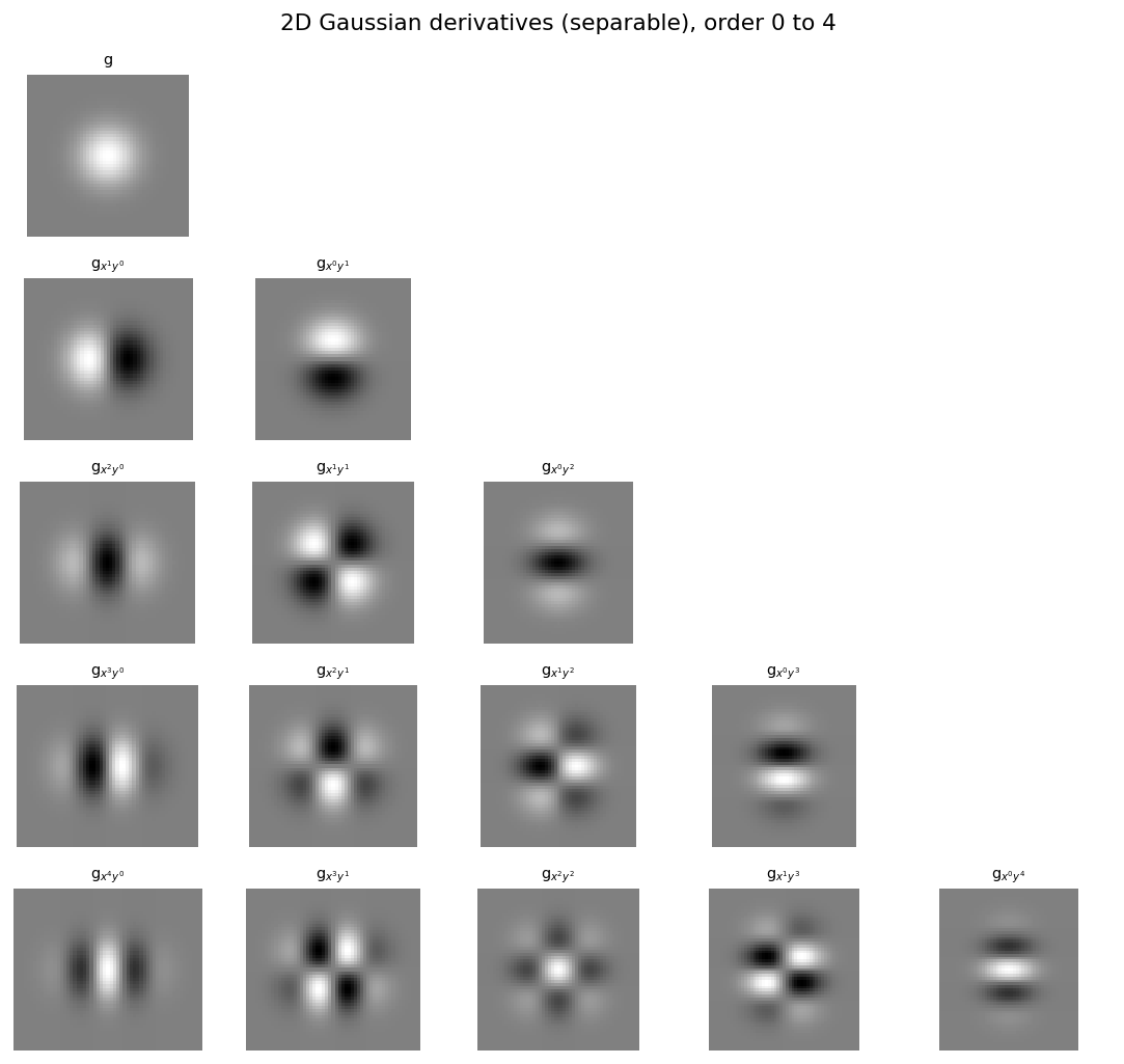
Because the 2-D Gaussian is **separable**, every mixed partial $g_{x^n y^m}$ is just the outer product of two 1-D Hermite-weighted Gaussians. Arranged by total order they form a triangle (the top is $g$ itself; each row adds one derivative). Each kernel is shown signed around mid-gray. These are exactly the oriented center-surround filters a linear front-end computes.
```python theme={null}
# Figure 18.10: triangle of separable 2D Gaussian derivatives, order 0..4.
K = 4; sig = 6.0
```
```python theme={null}
# Sanity: order-0 integrates to ~1 (unit area); every derivative integrates to ~0.
for n in range(4):
print(f'sum of order {n}:', float(dgauss_1d(1.0, n, radius=8).sum()))
```
```output theme={null}
sum of order 0: 1.0
sum of order 1: 0.0
sum of order 2: -2.3798011739017966e-07
sum of order 3: 0.0
```
### The 2-D Gaussian-derivative triangle
Because the 2-D Gaussian is **separable**, every mixed partial $g_{x^n y^m}$ is just the outer product of two 1-D Hermite-weighted Gaussians. Arranged by total order they form a triangle (the top is $g$ itself; each row adds one derivative). Each kernel is shown signed around mid-gray. These are exactly the oriented center-surround filters a linear front-end computes.
```python theme={null}
# Figure 18.10: triangle of separable 2D Gaussian derivatives, order 0..4.
K = 4; sig = 6.0
```
 ### Multiscale Gaussian derivatives
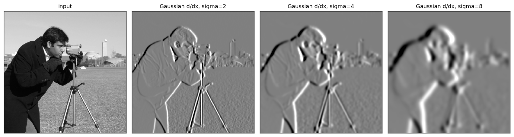
The scale $\sigma$ selects which edges survive: small $\sigma$ picks up fine texture, large $\sigma$ only the coarse structure. Here is the Gaussian x-derivative of a photograph at $\sigma=2,4,8$ (the book uses [a zebra](https://visionbook.mit.edu/derivatives.html#fig-gaussiander_zebra)).
```python theme={null}
# Figure 18.8: Gaussian x-derivative of a photo at increasing scale,
# shown signed around mid-gray (embossed edges), as in the book.
# stand-in for a photograph of a zebra in the book; original: https://visionbook.mit.edu/derivatives.html#fig-gaussiander_zebra
zebra = camera
panels, titles = [zebra], ['input']
for s in (2.0, 4.0, 8.0):
resp = conv2d(zebra, gauss_deriv2d(s, 1, 0))
panels.append(show_signed(resp)); titles.append(f'Gaussian d/dx, sigma={int(s)}')
```
### Multiscale Gaussian derivatives
The scale $\sigma$ selects which edges survive: small $\sigma$ picks up fine texture, large $\sigma$ only the coarse structure. Here is the Gaussian x-derivative of a photograph at $\sigma=2,4,8$ (the book uses [a zebra](https://visionbook.mit.edu/derivatives.html#fig-gaussiander_zebra)).
```python theme={null}
# Figure 18.8: Gaussian x-derivative of a photo at increasing scale,
# shown signed around mid-gray (embossed edges), as in the book.
# stand-in for a photograph of a zebra in the book; original: https://visionbook.mit.edu/derivatives.html#fig-gaussiander_zebra
zebra = camera
panels, titles = [zebra], ['input']
for s in (2.0, 4.0, 8.0):
resp = conv2d(zebra, gauss_deriv2d(s, 1, 0))
panels.append(show_signed(resp)); titles.append(f'Gaussian d/dx, sigma={int(s)}')
```
 ## Derivatives from binomial filters
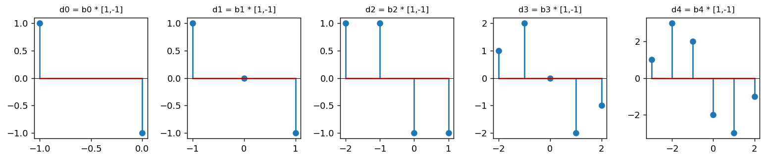
Convolving a binomial smoother $b_n$ (Pascal's triangle) with the elementary difference $[1,-1]$ gives a family of discrete derivative kernels $d_n=b_n*[1,-1]$: smoother as $n$ grows, all with DC gain 0.
$d_0=[1,-1],\quad d_1=[1,0,-1],\quad d_2=[1,1,-1,-1],\quad d_3=[1,2,0,-2,-1],\dots$
```python theme={null}
# The derivative-of-binomial family: d_n = b_n * [1, -1].
def binom(n):
b = np.array([1.0])
for _ in range(n):
b = np.convolve(b, [1.0, 1.0])
return b
```
```output theme={null}
d0: [ 1 -1] sum = 0
d1: [ 1 0 -1] sum = 0
d2: [ 1 1 -1 -1] sum = 0
d3: [ 1 2 0 -2 -1] sum = 0
d4: [ 1 3 2 -2 -3 -1] sum = 0
```
## Derivatives from binomial filters
Convolving a binomial smoother $b_n$ (Pascal's triangle) with the elementary difference $[1,-1]$ gives a family of discrete derivative kernels $d_n=b_n*[1,-1]$: smoother as $n$ grows, all with DC gain 0.
$d_0=[1,-1],\quad d_1=[1,0,-1],\quad d_2=[1,1,-1,-1],\quad d_3=[1,2,0,-2,-1],\dots$
```python theme={null}
# The derivative-of-binomial family: d_n = b_n * [1, -1].
def binom(n):
b = np.array([1.0])
for _ in range(n):
b = np.convolve(b, [1.0, 1.0])
return b
```
```output theme={null}
d0: [ 1 -1] sum = 0
d1: [ 1 0 -1] sum = 0
d2: [ 1 1 -1 -1] sum = 0
d3: [ 1 2 0 -2 -1] sum = 0
d4: [ 1 3 2 -2 -3 -1] sum = 0
```
 ### Roberts and Sobel in frequency
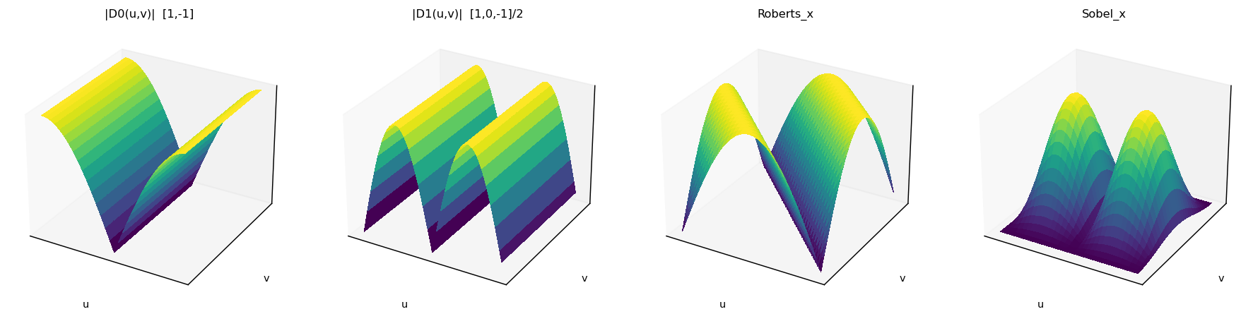
The **Roberts cross** ($2\times2$ diagonal differences) and the **Sobel-Feldman** operator ($[1,0,-1]$ derivative $\times$ $[1,2,1]$ smoothing) are the classic 2-D edge operators. Sobel is separable, $\text{Sobel}_x = [1,0,-1]\otimes[1,2,1]^\top$, and its smoothing makes it the most **isotropic and noise-tolerant**. The 2-D DFT magnitudes below show each operator's directional selectivity.
```python theme={null}
# Figure 18.14: 2D |DFT| SURFACES of d0, d1, Roberts_x, Sobel_x (as in the book).
def dft_mag(kernel, N=64):
k = np.zeros((N, N)); kh, kw = kernel.shape
k[:kh, :kw] = kernel # place at origin
return np.abs(np.fft.fftshift(np.fft.fft2(k)))
kernels = {
'|D0(u,v)| [1,-1]': np.array([[1.0, -1.0]]),
'|D1(u,v)| [1,0,-1]/2': np.array([[1.0, 0.0, -1.0]]) / 2,
'Roberts_x': np.array([[1.0, 0.0], [0.0, -1.0]]),
'Sobel_x': np.array([[1.0, 0.0, -1.0], [2.0, 0.0, -2.0], [1.0, 0.0, -1.0]]),
}
uv = np.linspace(-0.5, 0.5, 64)
U, V = np.meshgrid(uv, uv)
```
### Roberts and Sobel in frequency
The **Roberts cross** ($2\times2$ diagonal differences) and the **Sobel-Feldman** operator ($[1,0,-1]$ derivative $\times$ $[1,2,1]$ smoothing) are the classic 2-D edge operators. Sobel is separable, $\text{Sobel}_x = [1,0,-1]\otimes[1,2,1]^\top$, and its smoothing makes it the most **isotropic and noise-tolerant**. The 2-D DFT magnitudes below show each operator's directional selectivity.
```python theme={null}
# Figure 18.14: 2D |DFT| SURFACES of d0, d1, Roberts_x, Sobel_x (as in the book).
def dft_mag(kernel, N=64):
k = np.zeros((N, N)); kh, kw = kernel.shape
k[:kh, :kw] = kernel # place at origin
return np.abs(np.fft.fftshift(np.fft.fft2(k)))
kernels = {
'|D0(u,v)| [1,-1]': np.array([[1.0, -1.0]]),
'|D1(u,v)| [1,0,-1]/2': np.array([[1.0, 0.0, -1.0]]) / 2,
'Roberts_x': np.array([[1.0, 0.0], [0.0, -1.0]]),
'Sobel_x': np.array([[1.0, 0.0, -1.0], [2.0, 0.0, -2.0], [1.0, 0.0, -1.0]]),
}
uv = np.linspace(-0.5, 0.5, 64)
U, V = np.meshgrid(uv, uv)
```
 ## Image gradient and directional derivatives
The gradient $\nabla\ell=(\partial_x\ell,\partial_y\ell)$ is a per-pixel vector. The derivative in any direction $\mathbf t=(\cos\theta,\sin\theta)$ is just a linear combination of the two you already have, with **no new convolution needed**:
$\frac{\partial\ell}{\partial\mathbf t} = \cos\theta\,\partial_x\ell + \sin\theta\,\partial_y\ell.$
```python theme={null}
# Figure 18.15: directional derivatives of a disc: d/dx, d/dy, d/d45, plus the
# gradient magnitude |grad I| and the gradient ORIENTATION as a color wheel
# (hue = angle), exactly as the book lays it out.
import math
import matplotlib.colors as mcolors
yy, xx = torch.meshgrid(torch.linspace(-1, 1, 256), torch.linspace(-1, 1, 256), indexing='ij')
disc = (xx**2 + yy**2 < 0.5**2).float()
smooth = torch.outer(gaussian_1d(2.0), gaussian_1d(2.0)) # anti-alias the hard edge
disc = conv2d(disc, smooth)
dx = conv2d(disc, D1); dy = conv2d(disc, D1.T)
d45 = math.cos(math.pi / 4) * dx + math.sin(math.pi / 4) * dy
mag = torch.sqrt(dx**2 + dy**2)
ang = torch.atan2(dy, dx) # -pi .. pi
hue = ((ang / (2 * math.pi)) % 1.0).numpy() # 0 .. 1
val = (mag / mag.max()).clamp(0, 1).numpy() ** 0.5 # brightness = edge strength
angle_rgb = mcolors.hsv_to_rgb(np.stack([hue, np.ones_like(hue), val], axis=-1))
```
## Image gradient and directional derivatives
The gradient $\nabla\ell=(\partial_x\ell,\partial_y\ell)$ is a per-pixel vector. The derivative in any direction $\mathbf t=(\cos\theta,\sin\theta)$ is just a linear combination of the two you already have, with **no new convolution needed**:
$\frac{\partial\ell}{\partial\mathbf t} = \cos\theta\,\partial_x\ell + \sin\theta\,\partial_y\ell.$
```python theme={null}
# Figure 18.15: directional derivatives of a disc: d/dx, d/dy, d/d45, plus the
# gradient magnitude |grad I| and the gradient ORIENTATION as a color wheel
# (hue = angle), exactly as the book lays it out.
import math
import matplotlib.colors as mcolors
yy, xx = torch.meshgrid(torch.linspace(-1, 1, 256), torch.linspace(-1, 1, 256), indexing='ij')
disc = (xx**2 + yy**2 < 0.5**2).float()
smooth = torch.outer(gaussian_1d(2.0), gaussian_1d(2.0)) # anti-alias the hard edge
disc = conv2d(disc, smooth)
dx = conv2d(disc, D1); dy = conv2d(disc, D1.T)
d45 = math.cos(math.pi / 4) * dx + math.sin(math.pi / 4) * dy
mag = torch.sqrt(dx**2 + dy**2)
ang = torch.atan2(dy, dx) # -pi .. pi
hue = ((ang / (2 * math.pi)) % 1.0).numpy() # 0 .. 1
val = (mag / mag.max()).clamp(0, 1).numpy() ** 0.5 # brightness = edge strength
angle_rgb = mcolors.hsv_to_rgb(np.stack([hue, np.ones_like(hue), val], axis=-1))
```
 ## The Laplacian and Laplacian-of-Gaussian
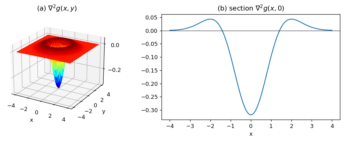
The **Laplacian** $\nabla^2\ell=\partial_{xx}\ell+\partial_{yy}\ell$ is the simplest **rotationally invariant** second-order operator. Smoothed with a Gaussian it becomes the **Laplacian-of-Gaussian** (the *Mexican-hat* wavelet),
$\nabla^2 g = \frac{x^2+y^2-2\sigma^2}{\sigma^4}\,g(x,y;\sigma),$
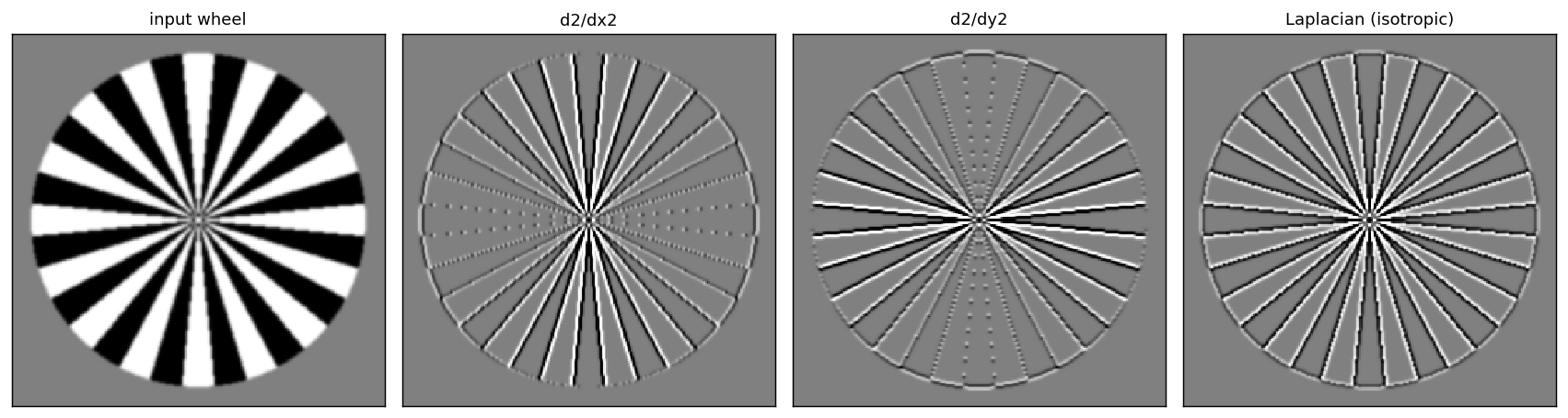
a center-surround kernel that responds to blobs and zero-crosses at edges. The book shows the second derivatives on [a photograph of a wheel](https://visionbook.mit.edu/derivatives.html#fig-wheellaplacian); below, a synthetic spoked wheel has edges at every orientation, which is what tests isotropy.
```python theme={null}
# Figure 18.16: Laplacian-of-Gaussian (Mexican hat), sigma = 1, x,y in [-4, 4].
# Plotted as grad^2 g (NOT negated): a well that dips to ~-0.3 with a positive rim.
xx = np.linspace(-4, 4, 121)
X, Y = np.meshgrid(xx, xx)
sig = 1.0
g = np.exp(-(X**2 + Y**2) / (2 * sig**2)) / (2 * np.pi * sig**2)
log = (X**2 + Y**2 - 2 * sig**2) / sig**4 * g # grad^2 g
```
## The Laplacian and Laplacian-of-Gaussian
The **Laplacian** $\nabla^2\ell=\partial_{xx}\ell+\partial_{yy}\ell$ is the simplest **rotationally invariant** second-order operator. Smoothed with a Gaussian it becomes the **Laplacian-of-Gaussian** (the *Mexican-hat* wavelet),
$\nabla^2 g = \frac{x^2+y^2-2\sigma^2}{\sigma^4}\,g(x,y;\sigma),$
a center-surround kernel that responds to blobs and zero-crosses at edges. The book shows the second derivatives on [a photograph of a wheel](https://visionbook.mit.edu/derivatives.html#fig-wheellaplacian); below, a synthetic spoked wheel has edges at every orientation, which is what tests isotropy.
```python theme={null}
# Figure 18.16: Laplacian-of-Gaussian (Mexican hat), sigma = 1, x,y in [-4, 4].
# Plotted as grad^2 g (NOT negated): a well that dips to ~-0.3 with a positive rim.
xx = np.linspace(-4, 4, 121)
X, Y = np.meshgrid(xx, xx)
sig = 1.0
g = np.exp(-(X**2 + Y**2) / (2 * sig**2)) / (2 * np.pi * sig**2)
log = (X**2 + Y**2 - 2 * sig**2) / sig**4 * g # grad^2 g
```
 ```python theme={null}
# Figure 18.18: second derivatives of a spoked wheel: d2/dx2, d2/dy2, and their sum
# (the Laplacian) is rotationally invariant. Five-point stencil:
# [[0,1,0],[1,-4,1],[0,1,0]].
wy, wx = torch.meshgrid(torch.linspace(-1, 1, 256), torch.linspace(-1, 1, 256), indexing='ij')
# stand-in for a photograph of a wheel in the book; original: https://visionbook.mit.edu/figures/spatial_filters/wheel256.jpg
spokes = (torch.cos(16 * torch.atan2(wy, wx)) > 0).float() # 16 spokes
wheel = torch.where(wx**2 + wy**2 < 0.9**2, 0.15 + 0.7 * spokes, torch.full_like(wx, 0.5))
wheel = conv2d(wheel, torch.outer(gaussian_1d(1.0), gaussian_1d(1.0))) # soften aliasing
dxx = conv2d(wheel, torch.tensor([[1.0, -2.0, 1.0]])) # d2/dx2
dyy = conv2d(wheel, torch.tensor([[1.0], [-2.0], [1.0]])) # d2/dy2
lap = conv2d(wheel, torch.tensor([[0., 1., 0.], [1., -4., 1.], [0., 1., 0.]]))
```
```python theme={null}
# Figure 18.18: second derivatives of a spoked wheel: d2/dx2, d2/dy2, and their sum
# (the Laplacian) is rotationally invariant. Five-point stencil:
# [[0,1,0],[1,-4,1],[0,1,0]].
wy, wx = torch.meshgrid(torch.linspace(-1, 1, 256), torch.linspace(-1, 1, 256), indexing='ij')
# stand-in for a photograph of a wheel in the book; original: https://visionbook.mit.edu/figures/spatial_filters/wheel256.jpg
spokes = (torch.cos(16 * torch.atan2(wy, wx)) > 0).float() # 16 spokes
wheel = torch.where(wx**2 + wy**2 < 0.9**2, 0.15 + 0.7 * spokes, torch.full_like(wx, 0.5))
wheel = conv2d(wheel, torch.outer(gaussian_1d(1.0), gaussian_1d(1.0))) # soften aliasing
dxx = conv2d(wheel, torch.tensor([[1.0, -2.0, 1.0]])) # d2/dx2
dyy = conv2d(wheel, torch.tensor([[1.0], [-2.0], [1.0]])) # d2/dy2
lap = conv2d(wheel, torch.tensor([[0., 1., 0.], [1., -4., 1.], [0., 1., 0.]]))
```
 ```python theme={null}
print('max |dxx+dyy - Laplacian|:', (dxx + dyy - lap).abs().max().item())
```
```output theme={null}
max |dxx+dyy - Laplacian|: 1.1920928955078125e-07
```
## Sharpening: unsharp masking
Subtracting a blurred copy from twice the image boosts the high frequencies the blur removed:
$\text{sharpen} = 2\mathbf I - b_{2,2},\qquad \text{DC gain} = 1.$
Applied repeatedly it keeps enhancing edges (until artifacts appear). The photo is in color, so the sharpen kernel is applied to each channel independently. The book uses [a photograph of a boat](https://visionbook.mit.edu/derivatives.html#fig-convExamps3).
```python theme={null}
# Figure 18.23: unsharp masking applied 1..5 times to a color photo.
# stand-in for a photograph of a boat in the book; original: https://visionbook.mit.edu/figures/spatial_filters/boat_sharp0.jpg
boat = coffee_rgb
b = torch.tensor([1.0, 2.0, 1.0]); blur = torch.outer(b, b); blur = blur / blur.sum()
sharpen = torch.zeros(3, 3); sharpen[1, 1] = 2.0; sharpen = sharpen - blur # 2I - b22
panels, titles = [boat], ['original']
cur = boat
for i in range(1, 6):
cur = conv2d_rgb(cur, sharpen).clamp(0, 1)
panels.append(cur); titles.append(f'sharpen x{i}')
```
```python theme={null}
print('max |dxx+dyy - Laplacian|:', (dxx + dyy - lap).abs().max().item())
```
```output theme={null}
max |dxx+dyy - Laplacian|: 1.1920928955078125e-07
```
## Sharpening: unsharp masking
Subtracting a blurred copy from twice the image boosts the high frequencies the blur removed:
$\text{sharpen} = 2\mathbf I - b_{2,2},\qquad \text{DC gain} = 1.$
Applied repeatedly it keeps enhancing edges (until artifacts appear). The photo is in color, so the sharpen kernel is applied to each channel independently. The book uses [a photograph of a boat](https://visionbook.mit.edu/derivatives.html#fig-convExamps3).
```python theme={null}
# Figure 18.23: unsharp masking applied 1..5 times to a color photo.
# stand-in for a photograph of a boat in the book; original: https://visionbook.mit.edu/figures/spatial_filters/boat_sharp0.jpg
boat = coffee_rgb
b = torch.tensor([1.0, 2.0, 1.0]); blur = torch.outer(b, b); blur = blur / blur.sum()
sharpen = torch.zeros(3, 3); sharpen[1, 1] = 2.0; sharpen = sharpen - blur # 2I - b22
panels, titles = [boat], ['original']
cur = boat
for i in range(1, 6):
cur = conv2d_rgb(cur, sharpen).clamp(0, 1)
panels.append(cur); titles.append(f'sharpen x{i}')
```
 ```python theme={null}
print('sharpen kernel DC gain:', float(sharpen.sum()))
```
```output theme={null}
sharpen kernel DC gain: 1.0
```
## Retinex: separating reflectance from illumination
An image is reflectance times illumination, $\ell=r\cdot l$. In the log domain this is a sum, and Land's **Retinex** exploits a statistical gap: **reflectance edges are sharp (large log-gradients)** while **illumination varies smoothly (small gradients)**. So you threshold the log-gradient: keep the large part as reflectance, integrate it back with a (mirror-padded) Poisson solve, and take the smooth remainder as illumination.
The test setup follows the book: a **synthetic Mondrian** (piecewise-constant reflectance patches) under a **smooth, left-bright illumination**, laid out as the book's $\ell(x,y)=r(x,y)\cdot l(x,y)$ decomposition. Because the ground truth is known, you can *measure* the recovery: the smooth **illumination is recovered almost exactly** (correlation \~0.97), and the **reflectance** comes out flat (\~0.77; the residual is faint illumination the single global threshold cannot fully separate).
```python theme={null}
# Figure 18.25/26: Retinex on a synthetic Mondrian x smooth illumination,
# laid out as the book's l(x,y) = r(x,y) x l(x,y) decomposition.
def fdx(a): return torch.roll(a, -1, dims=1) - a # forward difference f[n+1]-f[n]
def fdy(a): return torch.roll(a, -1, dims=0) - a
def poisson_periodic(gx, gy):
H, W = gx.shape
fy = np.fft.fftfreq(H)[:, None]; fx = np.fft.fftfreq(W)[None, :]
Dx = np.exp(2j * np.pi * fx) - 1; Dy = np.exp(2j * np.pi * fy) - 1
Gx = np.fft.fft2(gx); Gy = np.fft.fft2(gy)
denom = np.abs(Dx)**2 + np.abs(Dy)**2; denom[0, 0] = 1.0
Fh = (np.conj(Dx) * Gx + np.conj(Dy) * Gy) / denom; Fh[0, 0] = 0.0
return np.real(np.fft.ifft2(Fh))
def integrate(gx, gy):
"""Integrate a gradient field. The gradients are MIRROR-reflected first so the
periodic FFT solve behaves like a Neumann boundary, without this the recovered
reflectance keeps a low-frequency illumination ramp.
"""
gx = gx.numpy(); gy = gy.numpy(); H, W = gx.shape
GX = np.block([[gx, -gx[:, ::-1]], [gx[::-1, :], -gx[::-1, ::-1]]])
GY = np.block([[gy, gy[:, ::-1]], [-gy[::-1, :], -gy[::-1, ::-1]]])
f = poisson_periodic(GX, GY)[:H, :W]
return torch.tensor(f, dtype=torch.float32)
def corr(a, b):
a = a.flatten() - a.mean(); b = b.flatten() - b.mean()
return (a * b).sum() / (a.norm() * b.norm() + 1e-12)
# Ground truth: a rich Mondrian (distinct gray levels) under a smooth,
# left-bright illumination, the book's test image.
_ = torch.manual_seed(7)
gyN, gxN, ps = 8, 16, 18
H, Wd = gyN * ps, gxN * ps # 144 x 288, wide like the book
levels = torch.tensor([0.18, 0.32, 0.46, 0.60, 0.74, 0.90])
patch = levels[torch.randint(0, len(levels), (gyN, gxN))]
R_true = patch.repeat_interleave(ps, 0).repeat_interleave(ps, 1)
yy, xx = torch.meshgrid(torch.linspace(0, 1, H), torch.linspace(0, 1, Wd), indexing='ij')
L_true = 0.18 + 0.82 * torch.exp(-(((xx - 0.16)**2) / (2 * 0.22**2)
+ ((yy - 0.40)**2) / (2 * 0.50**2)))
ell = (R_true * L_true).clamp(1e-3, 1.0)
# Retinex: threshold log-gradients, keep the sharp (reflectance) part, integrate.
logL = torch.log(ell)
gx, gy = fdx(logL), fdy(logL)
T = torch.quantile(torch.stack([gx.abs(), gy.abs()]).flatten(), 0.86)
gxr = torch.where(gx.abs() > T, gx, torch.zeros_like(gx))
gyr = torch.where(gy.abs() > T, gy, torch.zeros_like(gy))
logR = integrate(gxr, gyr); logR = logR - logR.mean() + logL.mean()
R_hat = torch.exp(logR).clamp(0, 2)
L_hat = ell / (R_hat + 1e-3) # illumination = smooth remainder
```
```python theme={null}
print('sharpen kernel DC gain:', float(sharpen.sum()))
```
```output theme={null}
sharpen kernel DC gain: 1.0
```
## Retinex: separating reflectance from illumination
An image is reflectance times illumination, $\ell=r\cdot l$. In the log domain this is a sum, and Land's **Retinex** exploits a statistical gap: **reflectance edges are sharp (large log-gradients)** while **illumination varies smoothly (small gradients)**. So you threshold the log-gradient: keep the large part as reflectance, integrate it back with a (mirror-padded) Poisson solve, and take the smooth remainder as illumination.
The test setup follows the book: a **synthetic Mondrian** (piecewise-constant reflectance patches) under a **smooth, left-bright illumination**, laid out as the book's $\ell(x,y)=r(x,y)\cdot l(x,y)$ decomposition. Because the ground truth is known, you can *measure* the recovery: the smooth **illumination is recovered almost exactly** (correlation \~0.97), and the **reflectance** comes out flat (\~0.77; the residual is faint illumination the single global threshold cannot fully separate).
```python theme={null}
# Figure 18.25/26: Retinex on a synthetic Mondrian x smooth illumination,
# laid out as the book's l(x,y) = r(x,y) x l(x,y) decomposition.
def fdx(a): return torch.roll(a, -1, dims=1) - a # forward difference f[n+1]-f[n]
def fdy(a): return torch.roll(a, -1, dims=0) - a
def poisson_periodic(gx, gy):
H, W = gx.shape
fy = np.fft.fftfreq(H)[:, None]; fx = np.fft.fftfreq(W)[None, :]
Dx = np.exp(2j * np.pi * fx) - 1; Dy = np.exp(2j * np.pi * fy) - 1
Gx = np.fft.fft2(gx); Gy = np.fft.fft2(gy)
denom = np.abs(Dx)**2 + np.abs(Dy)**2; denom[0, 0] = 1.0
Fh = (np.conj(Dx) * Gx + np.conj(Dy) * Gy) / denom; Fh[0, 0] = 0.0
return np.real(np.fft.ifft2(Fh))
def integrate(gx, gy):
"""Integrate a gradient field. The gradients are MIRROR-reflected first so the
periodic FFT solve behaves like a Neumann boundary, without this the recovered
reflectance keeps a low-frequency illumination ramp.
"""
gx = gx.numpy(); gy = gy.numpy(); H, W = gx.shape
GX = np.block([[gx, -gx[:, ::-1]], [gx[::-1, :], -gx[::-1, ::-1]]])
GY = np.block([[gy, gy[:, ::-1]], [-gy[::-1, :], -gy[::-1, ::-1]]])
f = poisson_periodic(GX, GY)[:H, :W]
return torch.tensor(f, dtype=torch.float32)
def corr(a, b):
a = a.flatten() - a.mean(); b = b.flatten() - b.mean()
return (a * b).sum() / (a.norm() * b.norm() + 1e-12)
# Ground truth: a rich Mondrian (distinct gray levels) under a smooth,
# left-bright illumination, the book's test image.
_ = torch.manual_seed(7)
gyN, gxN, ps = 8, 16, 18
H, Wd = gyN * ps, gxN * ps # 144 x 288, wide like the book
levels = torch.tensor([0.18, 0.32, 0.46, 0.60, 0.74, 0.90])
patch = levels[torch.randint(0, len(levels), (gyN, gxN))]
R_true = patch.repeat_interleave(ps, 0).repeat_interleave(ps, 1)
yy, xx = torch.meshgrid(torch.linspace(0, 1, H), torch.linspace(0, 1, Wd), indexing='ij')
L_true = 0.18 + 0.82 * torch.exp(-(((xx - 0.16)**2) / (2 * 0.22**2)
+ ((yy - 0.40)**2) / (2 * 0.50**2)))
ell = (R_true * L_true).clamp(1e-3, 1.0)
# Retinex: threshold log-gradients, keep the sharp (reflectance) part, integrate.
logL = torch.log(ell)
gx, gy = fdx(logL), fdy(logL)
T = torch.quantile(torch.stack([gx.abs(), gy.abs()]).flatten(), 0.86)
gxr = torch.where(gx.abs() > T, gx, torch.zeros_like(gx))
gyr = torch.where(gy.abs() > T, gy, torch.zeros_like(gy))
logR = integrate(gxr, gyr); logR = logR - logR.mean() + logL.mean()
R_hat = torch.exp(logR).clamp(0, 2)
L_hat = ell / (R_hat + 1e-3) # illumination = smooth remainder
```
 ```python theme={null}
print('corr(recovered reflectance, truth):', corr(R_hat, R_true).item())
print('corr(recovered illumination, truth):', corr(L_hat, L_true).item())
```
```output theme={null}
corr(recovered reflectance, truth): 0.7698575854301453
corr(recovered illumination, truth): 0.9723199605941772
```
## Concluding remarks
| Operator | Kernel | Property |
| - | - | - |
| two-tap $d_0$ | $[1,-1]$ | half-pixel shift, widest band |
| centered $d_1$ | $[1,0,-1]/2$ | no shift, smoother |
| Gaussian deriv | $-\tfrac{x}{\sigma^2}g$ | smooths + differentiates; scale-selective |
| Sobel | $[1,0,-1]\otimes[1,2,1]$ | separable, isotropic, noise-tolerant |
| Laplacian | $[[0,1,0],[1,-4,1],[0,1,0]]$ | rotationally invariant, zero-crossings at edges |
| sharpen | $2\mathbf I - b_{2,2}$ | high-boost, DC gain 1 |
From a single idea, differencing neighboring pixels, the chapter builds edge detection, scale selection (Gaussian derivatives), the isotropic Laplacian, sharpening, and gradient-domain reasoning strong enough to **separate reflectance from illumination**. These operators are the front end of nearly every classical vision pipeline (SIFT, HOG) and echo the center-surround receptive fields of early biological vision.
***
[Edit this page on GitHub](https://github.com/aegean-ai/eaia/edit/main/src/aiml-common/lectures/image-processing/image-derivatives/index.mdx) or [file an issue](https://github.com/aegean-ai/eaia/issues/new/choose).
```python theme={null}
print('corr(recovered reflectance, truth):', corr(R_hat, R_true).item())
print('corr(recovered illumination, truth):', corr(L_hat, L_true).item())
```
```output theme={null}
corr(recovered reflectance, truth): 0.7698575854301453
corr(recovered illumination, truth): 0.9723199605941772
```
## Concluding remarks
| Operator | Kernel | Property |
| - | - | - |
| two-tap $d_0$ | $[1,-1]$ | half-pixel shift, widest band |
| centered $d_1$ | $[1,0,-1]/2$ | no shift, smoother |
| Gaussian deriv | $-\tfrac{x}{\sigma^2}g$ | smooths + differentiates; scale-selective |
| Sobel | $[1,0,-1]\otimes[1,2,1]$ | separable, isotropic, noise-tolerant |
| Laplacian | $[[0,1,0],[1,-4,1],[0,1,0]]$ | rotationally invariant, zero-crossings at edges |
| sharpen | $2\mathbf I - b_{2,2}$ | high-boost, DC gain 1 |
From a single idea, differencing neighboring pixels, the chapter builds edge detection, scale selection (Gaussian derivatives), the isotropic Laplacian, sharpening, and gradient-domain reasoning strong enough to **separate reflectance from illumination**. These operators are the front end of nearly every classical vision pipeline (SIFT, HOG) and echo the center-surround receptive fields of early biological vision.
***
[Edit this page on GitHub](https://github.com/aegean-ai/eaia/edit/main/src/aiml-common/lectures/image-processing/image-derivatives/index.mdx) or [file an issue](https://github.com/aegean-ai/eaia/issues/new/choose).