> ## Documentation Index
> Fetch the complete documentation index at: https://aegean.ai/llms.txt
> Use this file to discover all available pages before exploring further.
# Sampling an Image Without Aliasing
> The sampling theorem, aliasing in 1D and 2D, sinc and local reconstruction, sampling lattices, and anti-aliasing filters.
 *This section was written by [Nazib Khan](https://github.com/Nazib65) ([pull request #46](https://github.com/pantelis/eng-ai-agents/pull/46)), with help from an AI coding agent on the code. It reproduces the ideas of Chapter 20 of [*Foundations of Computer Vision*](https://visionbook.mit.edu/sampling_and_aliasing.html) by Antonio Torralba, Phillip Isola, and William T. Freeman. The book's own figures are not reproduced here, because the book's license covers only the work in full; links point to them instead.*
This section regenerates the figures of the book's sampling chapter in PyTorch. Change a parameter in any cell and its figure updates.
**The thread through the section.** Sampling keeps a continuous signal only at instants spaced by $T_s = 1/f_s$. Frequencies separated by a whole multiple of $f_s$ then leave *identical* samples, so the original is no longer recoverable: this is **aliasing**. The **sampling theorem** says aliasing is avoided exactly when $f_s > 2 f_{\max}$ (the Nyquist rate). **Reconstruction** fills the gaps between samples, and an **anti-aliasing filter** band-limits a signal before sampling so the theorem can be honored.
Figure 20.15, the cone mosaic of the primate fovea, is a micrograph rather than a computed plot, so a link points to it.
```python theme={null}
# Every signal in this section is a tensor; a fixed seed keeps the figures reproducible.
import math
import torch
import matplotlib.pyplot as plt
import kornia
from skimage.data import camera
_ = torch.manual_seed(0)
DEVICE = "cuda" if torch.cuda.is_available() else "cpu"
# A dense grid over [0, 1] stands in for the continuous-time axis in the 1-D figures.
t_cont = torch.linspace(0, 1, 2000, device=DEVICE)
print(f"torch {torch.__version__} on {DEVICE} | kornia {kornia.__version__}")
```
```output theme={null}
torch 2.11.0+cu130 on cpu | kornia 0.8.3
```
**Images replaced for licensing.** The book is published under a CC BY-NC-ND license, which covers only the book as a whole and not its individual images, so this page does not republish the book's photographs. License-free images stand in for them:
* The *cameraman* photograph (scikit-image) stands in for [a photograph of a zebra (Figure 20.16)](https://visionbook.mit.edu/sampling_and_aliasing.html#fig-aliasingFTzebra).
If you use the book for non-commercial purposes, you can swap the originals back in: each line that loads a stand-in carries the original's link in a comment.
## Figure 20.1: the continuous wave
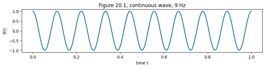
The input is a cosine $\ell(t) = \cos(\omega t)$ with radian frequency $\omega = 18\pi$,
i.e. an ordinary frequency of $\omega/2\pi = 9$ Hz, completing nine cycles over the unit
interval. This is the signal that sampling has to capture.
```python theme={null}
# Continuous input wave: cos(omega t) with omega = 18*pi -> 9 cycles over [0, 1].
omega = 18 * math.pi # radian frequency used by the book
f_in = omega / (2 * math.pi) # = 9 Hz, the ordinary frequency
wave_in = torch.cos(omega * t_cont)
print(f"input frequency: {f_in:.0f} Hz")
```
```output theme={null}
input frequency: 9 Hz
```
*This section was written by [Nazib Khan](https://github.com/Nazib65) ([pull request #46](https://github.com/pantelis/eng-ai-agents/pull/46)), with help from an AI coding agent on the code. It reproduces the ideas of Chapter 20 of [*Foundations of Computer Vision*](https://visionbook.mit.edu/sampling_and_aliasing.html) by Antonio Torralba, Phillip Isola, and William T. Freeman. The book's own figures are not reproduced here, because the book's license covers only the work in full; links point to them instead.*
This section regenerates the figures of the book's sampling chapter in PyTorch. Change a parameter in any cell and its figure updates.
**The thread through the section.** Sampling keeps a continuous signal only at instants spaced by $T_s = 1/f_s$. Frequencies separated by a whole multiple of $f_s$ then leave *identical* samples, so the original is no longer recoverable: this is **aliasing**. The **sampling theorem** says aliasing is avoided exactly when $f_s > 2 f_{\max}$ (the Nyquist rate). **Reconstruction** fills the gaps between samples, and an **anti-aliasing filter** band-limits a signal before sampling so the theorem can be honored.
Figure 20.15, the cone mosaic of the primate fovea, is a micrograph rather than a computed plot, so a link points to it.
```python theme={null}
# Every signal in this section is a tensor; a fixed seed keeps the figures reproducible.
import math
import torch
import matplotlib.pyplot as plt
import kornia
from skimage.data import camera
_ = torch.manual_seed(0)
DEVICE = "cuda" if torch.cuda.is_available() else "cpu"
# A dense grid over [0, 1] stands in for the continuous-time axis in the 1-D figures.
t_cont = torch.linspace(0, 1, 2000, device=DEVICE)
print(f"torch {torch.__version__} on {DEVICE} | kornia {kornia.__version__}")
```
```output theme={null}
torch 2.11.0+cu130 on cpu | kornia 0.8.3
```
**Images replaced for licensing.** The book is published under a CC BY-NC-ND license, which covers only the book as a whole and not its individual images, so this page does not republish the book's photographs. License-free images stand in for them:
* The *cameraman* photograph (scikit-image) stands in for [a photograph of a zebra (Figure 20.16)](https://visionbook.mit.edu/sampling_and_aliasing.html#fig-aliasingFTzebra).
If you use the book for non-commercial purposes, you can swap the originals back in: each line that loads a stand-in carries the original's link in a comment.
## Figure 20.1: the continuous wave
The input is a cosine $\ell(t) = \cos(\omega t)$ with radian frequency $\omega = 18\pi$,
i.e. an ordinary frequency of $\omega/2\pi = 9$ Hz, completing nine cycles over the unit
interval. This is the signal that sampling has to capture.
```python theme={null}
# Continuous input wave: cos(omega t) with omega = 18*pi -> 9 cycles over [0, 1].
omega = 18 * math.pi # radian frequency used by the book
f_in = omega / (2 * math.pi) # = 9 Hz, the ordinary frequency
wave_in = torch.cos(omega * t_cont)
print(f"input frequency: {f_in:.0f} Hz")
```
```output theme={null}
input frequency: 9 Hz
```
 ## Figure 20.2: sampling the wave
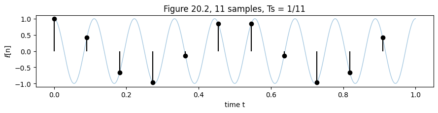
Sample with period $T_s = 1/11$, giving 11 samples across the interval. With 11 samples
for 9 periods it *seems* sufficient, with more samples than periods, yet Nyquist needs
$f_s > 18$. The block records the samples $\ell[n] = \ell(n T_s)$.
```python theme={null}
# Sample the wave on a coarse grid: period Ts = 1/11 -> 11 instants n*Ts.
fs = 11.0
t_samp = torch.arange(0, 1, 1.0 / fs, device=DEVICE)
samples = torch.cos(omega * t_samp)
print(f"{t_samp.numel()} samples for {f_in:.0f} periods; Nyquist needs fs > {2*f_in:.0f}")
```
```output theme={null}
11 samples for 9 periods; Nyquist needs fs > 18
```
## Figure 20.2: sampling the wave
Sample with period $T_s = 1/11$, giving 11 samples across the interval. With 11 samples
for 9 periods it *seems* sufficient, with more samples than periods, yet Nyquist needs
$f_s > 18$. The block records the samples $\ell[n] = \ell(n T_s)$.
```python theme={null}
# Sample the wave on a coarse grid: period Ts = 1/11 -> 11 instants n*Ts.
fs = 11.0
t_samp = torch.arange(0, 1, 1.0 / fs, device=DEVICE)
samples = torch.cos(omega * t_samp)
print(f"{t_samp.numel()} samples for {f_in:.0f} periods; Nyquist needs fs > {2*f_in:.0f}")
```
```output theme={null}
11 samples for 9 periods; Nyquist needs fs > 18
```
 ## Figure 20.3: many waves, the same samples
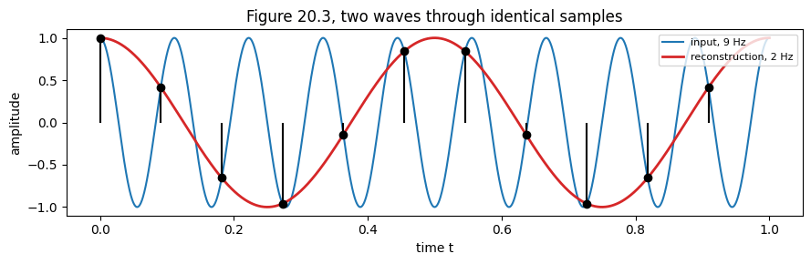
Reconstruction is ambiguous: nothing constrains the signal between samples. Under the
slow-and-smooth prior the reconstruction is the *slowest* cosine through the dots. Here
the 9 Hz input aliases to $|9 - 11| = 2$ Hz: subtracting one sampling rate gives the low
frequency that shares every sample, since
$\cos(2\pi\,9\,\tfrac{n}{11}) = \cos(2\pi\,(9-11)\tfrac{n}{11})$.
```python theme={null}
# The slow reconstruction: subtract one sampling rate, 9 - 11 = -2 Hz -> 2 Hz.
f_alias = abs(f_in - fs)
wave_recon = torch.cos(2 * math.pi * f_alias * t_cont)
# The 2 Hz reconstruction must match the 9 Hz input at every sample instant.
mismatch = (samples - torch.cos(2 * math.pi * f_alias * t_samp)).abs().max().item()
print(f"reconstruction {f_alias:.0f} Hz vs input {f_in:.0f} Hz: max |mismatch| = {mismatch:.1e}")
```
```output theme={null}
reconstruction 2 Hz vs input 9 Hz: max |mismatch| = 3.3e-06
```
## Figure 20.3: many waves, the same samples
Reconstruction is ambiguous: nothing constrains the signal between samples. Under the
slow-and-smooth prior the reconstruction is the *slowest* cosine through the dots. Here
the 9 Hz input aliases to $|9 - 11| = 2$ Hz: subtracting one sampling rate gives the low
frequency that shares every sample, since
$\cos(2\pi\,9\,\tfrac{n}{11}) = \cos(2\pi\,(9-11)\tfrac{n}{11})$.
```python theme={null}
# The slow reconstruction: subtract one sampling rate, 9 - 11 = -2 Hz -> 2 Hz.
f_alias = abs(f_in - fs)
wave_recon = torch.cos(2 * math.pi * f_alias * t_cont)
# The 2 Hz reconstruction must match the 9 Hz input at every sample instant.
mismatch = (samples - torch.cos(2 * math.pi * f_alias * t_samp)).abs().max().item()
print(f"reconstruction {f_alias:.0f} Hz vs input {f_in:.0f} Hz: max |mismatch| = {mismatch:.1e}")
```
```output theme={null}
reconstruction 2 Hz vs input 9 Hz: max |mismatch| = 3.3e-06
```
 ## Figure 20.4: aliasing bends a 2-D pattern
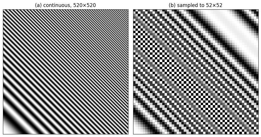
The 2-D analogue is $\ell(x,y) = \cos\!\big(2\pi\,a\,(x+y)^2\big)$: diagonal waves whose
frequency rises with $(x+y)^2$, slow at the bottom-left and ever finer toward the
top-right. Point-sampling to $52\times52$ with no pre-filter folds the unrepresentable
high frequencies back, and the dominant *orientation* of the stripes flips.
```python theme={null}
# Diagonal chirp: frequency grows with (x+y), so crests run diagonally and tighten.
N = 520
coords = torch.linspace(0, 1, N, device=DEVICE)
yy, xx = torch.meshgrid(coords, coords, indexing="ij")
pattern = torch.cos(2 * math.pi * 16 * (xx + yy) ** 2)
# Point-sample with no anti-alias pre-filter: keep every stride-th pixel, 520 -> 52.
stride = 10
aliased = pattern[::stride, ::stride]
print(f"continuous {tuple(pattern.shape)} -> point-sampled {tuple(aliased.shape)}")
```
```output theme={null}
continuous (520, 520) -> point-sampled (52, 52)
```
## Figure 20.4: aliasing bends a 2-D pattern
The 2-D analogue is $\ell(x,y) = \cos\!\big(2\pi\,a\,(x+y)^2\big)$: diagonal waves whose
frequency rises with $(x+y)^2$, slow at the bottom-left and ever finer toward the
top-right. Point-sampling to $52\times52$ with no pre-filter folds the unrepresentable
high frequencies back, and the dominant *orientation* of the stripes flips.
```python theme={null}
# Diagonal chirp: frequency grows with (x+y), so crests run diagonally and tighten.
N = 520
coords = torch.linspace(0, 1, N, device=DEVICE)
yy, xx = torch.meshgrid(coords, coords, indexing="ij")
pattern = torch.cos(2 * math.pi * 16 * (xx + yy) ** 2)
# Point-sample with no anti-alias pre-filter: keep every stride-th pixel, 520 -> 52.
stride = 10
aliased = pattern[::stride, ::stride]
print(f"continuous {tuple(pattern.shape)} -> point-sampled {tuple(aliased.shape)}")
```
```output theme={null}
continuous (520, 520) -> point-sampled (52, 52)
```
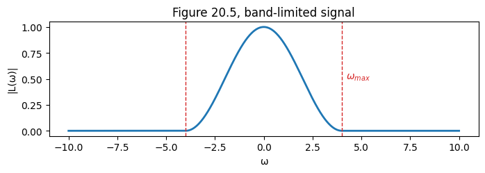
 ## Figure 20.5: a band-limited signal
The sampling theorem is stated for **band-limited** signals: those whose Fourier
transform $L(\omega)$ is zero above some maximum frequency $\omega_{\max}$. The sketch
below shows such a spectrum, nonzero only inside $[-\omega_{\max}, \omega_{\max}]$.
```python theme={null}
# A schematic band-limited spectrum |L(w)|: a smooth bump confined to |w| < w_max.
w = torch.linspace(-10, 10, 1000, device=DEVICE)
w_max = 4.0
spectrum = torch.where(w.abs() < w_max, torch.cos(math.pi * w / (2 * w_max)) ** 2,
torch.zeros_like(w))
print(f"spectrum support: |w| < w_max = {w_max}")
```
```output theme={null}
spectrum support: |w| < w_max = 4.0
```
## Figure 20.5: a band-limited signal
The sampling theorem is stated for **band-limited** signals: those whose Fourier
transform $L(\omega)$ is zero above some maximum frequency $\omega_{\max}$. The sketch
below shows such a spectrum, nonzero only inside $[-\omega_{\max}, \omega_{\max}]$.
```python theme={null}
# A schematic band-limited spectrum |L(w)|: a smooth bump confined to |w| < w_max.
w = torch.linspace(-10, 10, 1000, device=DEVICE)
w_max = 4.0
spectrum = torch.where(w.abs() < w_max, torch.cos(math.pi * w / (2 * w_max)) ** 2,
torch.zeros_like(w))
print(f"spectrum support: |w| < w_max = {w_max}")
```
```output theme={null}
spectrum support: |w| < w_max = 4.0
```
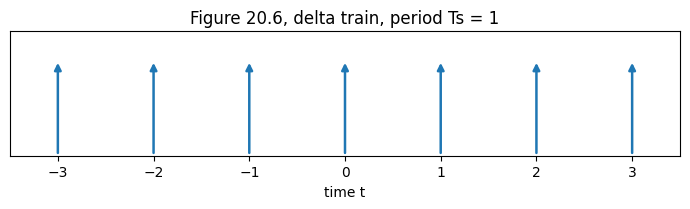
 ## Figure 20.6: the delta train
Sampling is modelled by multiplying the signal with a **delta train** (Dirac comb)
$\mathrm{III}(t) = \sum_n \delta(t - n T_s)$: impulses at every multiple of $T_s$. Here
$T_s = 1$. Arrow heads mark the impulses (each of infinite height, unit area).
```python theme={null}
# Delta train with period Ts = 1: impulse locations over a few periods.
Ts_comb = 1.0
impulse_times = torch.arange(-3, 4, Ts_comb)
print(f"impulses at t = {impulse_times.tolist()}")
```
```output theme={null}
impulses at t = [-3.0, -2.0, -1.0, 0.0, 1.0, 2.0, 3.0]
```
## Figure 20.6: the delta train
Sampling is modelled by multiplying the signal with a **delta train** (Dirac comb)
$\mathrm{III}(t) = \sum_n \delta(t - n T_s)$: impulses at every multiple of $T_s$. Here
$T_s = 1$. Arrow heads mark the impulses (each of infinite height, unit area).
```python theme={null}
# Delta train with period Ts = 1: impulse locations over a few periods.
Ts_comb = 1.0
impulse_times = torch.arange(-3, 4, Ts_comb)
print(f"impulses at t = {impulse_times.tolist()}")
```
```output theme={null}
impulses at t = [-3.0, -2.0, -1.0, 0.0, 1.0, 2.0, 3.0]
```
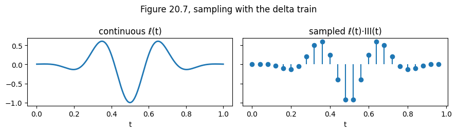
 ## Figure 20.7: sampling with the delta train
Multiplying a continuous signal by the delta train keeps its values only at the impulse
times, producing the sampled signal $\ell_s(t) = \ell(t)\,\mathrm{III}(t)$. Left: the
continuous signal. Right: its delta-sampled version, impulses scaled by the signal.
```python theme={null}
# A smooth low-frequency signal and its delta-train samples.
sig = torch.exp(-((t_cont - 0.5) ** 2) / 0.05) * torch.cos(2 * math.pi * 3 * t_cont)
Ts7 = 0.04
t7 = torch.arange(0, 1, Ts7, device=DEVICE)
sig7 = torch.exp(-((t7 - 0.5) ** 2) / 0.05) * torch.cos(2 * math.pi * 3 * t7)
print(f"continuous samples: {sig.numel()}, delta-train samples: {sig7.numel()}")
```
```output theme={null}
continuous samples: 2000, delta-train samples: 25
```
## Figure 20.7: sampling with the delta train
Multiplying a continuous signal by the delta train keeps its values only at the impulse
times, producing the sampled signal $\ell_s(t) = \ell(t)\,\mathrm{III}(t)$. Left: the
continuous signal. Right: its delta-sampled version, impulses scaled by the signal.
```python theme={null}
# A smooth low-frequency signal and its delta-train samples.
sig = torch.exp(-((t_cont - 0.5) ** 2) / 0.05) * torch.cos(2 * math.pi * 3 * t_cont)
Ts7 = 0.04
t7 = torch.arange(0, 1, Ts7, device=DEVICE)
sig7 = torch.exp(-((t7 - 0.5) ** 2) / 0.05) * torch.cos(2 * math.pi * 3 * t7)
print(f"continuous samples: {sig.numel()}, delta-train samples: {sig7.numel()}")
```
```output theme={null}
continuous samples: 2000, delta-train samples: 25
```
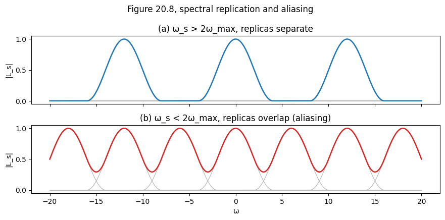
 ## Figure 20.8: aliasing in the Fourier domain
Sampling replicates the spectrum: the transform of the sampled signal is
$\sum_k L(\omega - k\,\omega_s)$, copies of $L$ spaced by the sampling frequency
$\omega_s$. **(a)** When $\omega_s > 2\omega_{\max}$ the copies stay separate and the
original is recoverable. **(b)** When $\omega_s < 2\omega_{\max}$ neighboring copies
overlap; high frequencies leak into low ones. That is aliasing.
```python theme={null}
# Replicate the band-limited bump at multiples of the sampling frequency w_s.
def replicate(w_axis, w_s, w_max, n=6):
total = torch.zeros_like(w_axis)
copies = []
for k in range(-n, n + 1):
shifted = w_axis - k * w_s
copy = torch.where(shifted.abs() < w_max,
torch.cos(math.pi * shifted / (2 * w_max)) ** 2,
torch.zeros_like(w_axis))
copies.append(copy); total = total + copy
return total, copies
w_axis = torch.linspace(-20, 20, 2000, device=DEVICE)
sep, sep_copies = replicate(w_axis, w_s=12.0, w_max=4.0) # w_s > 2 w_max -> no overlap
ovl, ovl_copies = replicate(w_axis, w_s=6.0, w_max=4.0) # w_s < 2 w_max -> overlap
print("case (a) w_s=12 > 8 : no overlap | case (b) w_s=6 < 8 : overlap")
```
```output theme={null}
case (a) w_s=12 > 8 : no overlap | case (b) w_s=6 < 8 : overlap
```
## Figure 20.8: aliasing in the Fourier domain
Sampling replicates the spectrum: the transform of the sampled signal is
$\sum_k L(\omega - k\,\omega_s)$, copies of $L$ spaced by the sampling frequency
$\omega_s$. **(a)** When $\omega_s > 2\omega_{\max}$ the copies stay separate and the
original is recoverable. **(b)** When $\omega_s < 2\omega_{\max}$ neighboring copies
overlap; high frequencies leak into low ones. That is aliasing.
```python theme={null}
# Replicate the band-limited bump at multiples of the sampling frequency w_s.
def replicate(w_axis, w_s, w_max, n=6):
total = torch.zeros_like(w_axis)
copies = []
for k in range(-n, n + 1):
shifted = w_axis - k * w_s
copy = torch.where(shifted.abs() < w_max,
torch.cos(math.pi * shifted / (2 * w_max)) ** 2,
torch.zeros_like(w_axis))
copies.append(copy); total = total + copy
return total, copies
w_axis = torch.linspace(-20, 20, 2000, device=DEVICE)
sep, sep_copies = replicate(w_axis, w_s=12.0, w_max=4.0) # w_s > 2 w_max -> no overlap
ovl, ovl_copies = replicate(w_axis, w_s=6.0, w_max=4.0) # w_s < 2 w_max -> overlap
print("case (a) w_s=12 > 8 : no overlap | case (b) w_s=6 < 8 : overlap")
```
```output theme={null}
case (a) w_s=12 > 8 : no overlap | case (b) w_s=6 < 8 : overlap
```
 ## Figure 20.9: the sinc function
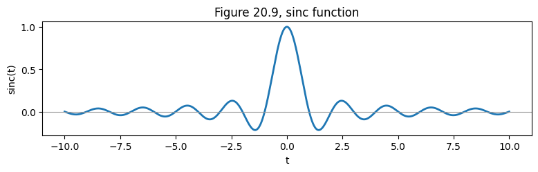
Ideal reconstruction convolves the samples with a $\mathrm{sinc}$, the impulse response
of the ideal low-pass (box) filter. $\mathrm{sinc}(t) = \sin(\pi t)/(\pi t)$ peaks at the
origin, is symmetric, and decays as $1/t$ with zero crossings at the integers.
```python theme={null}
# torch.sinc is the normalized sinc: sin(pi t)/(pi t), zero crossings at integers.
ts = torch.linspace(-10, 10, 2000, device=DEVICE)
sinc = torch.sinc(ts)
print(f"sinc(0) = {torch.sinc(torch.zeros(1)).item():.0f}, zero crossings at integers")
```
```output theme={null}
sinc(0) = 1, zero crossings at integers
```
## Figure 20.9: the sinc function
Ideal reconstruction convolves the samples with a $\mathrm{sinc}$, the impulse response
of the ideal low-pass (box) filter. $\mathrm{sinc}(t) = \sin(\pi t)/(\pi t)$ peaks at the
origin, is symmetric, and decays as $1/t$ with zero crossings at the integers.
```python theme={null}
# torch.sinc is the normalized sinc: sin(pi t)/(pi t), zero crossings at integers.
ts = torch.linspace(-10, 10, 2000, device=DEVICE)
sinc = torch.sinc(ts)
print(f"sinc(0) = {torch.sinc(torch.zeros(1)).item():.0f}, zero crossings at integers")
```
```output theme={null}
sinc(0) = 1, zero crossings at integers
```
 ## Figure 20.10: sinc interpolation
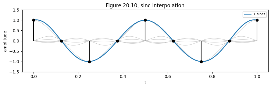
The ideal reconstruction is $\hat\ell(t) = \sum_n \ell[n]\,\mathrm{sinc}\!\big((t - nT_s)/T_s\big)$:
a scaled, shifted sinc centered on each sample. The thin curves are the individual sincs;
their sum (thick) is the smooth interpolation. Each sinc's zero crossings fall on the
*other* sample locations, so every sample is honoured exactly.
```python theme={null}
# Reconstruct a slow signal from its samples by summing shifted, scaled sincs.
Ts10 = 1.0 / 8
t10 = torch.arange(0, 1 + Ts10, Ts10, device=DEVICE)
x10 = torch.cos(2 * math.pi * 2 * t10) # samples of a 2 Hz wave
# Each sample contributes x[n]*sinc((t - n*Ts)/Ts); stack then sum over samples.
basis = x10[:, None] * torch.sinc((t_cont[None, :] - t10[:, None]) / Ts10)
recon10 = basis.sum(0)
print(f"{t10.numel()} samples reconstructed onto {t_cont.numel()} dense points")
```
```output theme={null}
9 samples reconstructed onto 2000 dense points
```
## Figure 20.10: sinc interpolation
The ideal reconstruction is $\hat\ell(t) = \sum_n \ell[n]\,\mathrm{sinc}\!\big((t - nT_s)/T_s\big)$:
a scaled, shifted sinc centered on each sample. The thin curves are the individual sincs;
their sum (thick) is the smooth interpolation. Each sinc's zero crossings fall on the
*other* sample locations, so every sample is honoured exactly.
```python theme={null}
# Reconstruct a slow signal from its samples by summing shifted, scaled sincs.
Ts10 = 1.0 / 8
t10 = torch.arange(0, 1 + Ts10, Ts10, device=DEVICE)
x10 = torch.cos(2 * math.pi * 2 * t10) # samples of a 2 Hz wave
# Each sample contributes x[n]*sinc((t - n*Ts)/Ts); stack then sum over samples.
basis = x10[:, None] * torch.sinc((t_cont[None, :] - t10[:, None]) / Ts10)
recon10 = basis.sum(0)
print(f"{t10.numel()} samples reconstructed onto {t_cont.numel()} dense points")
```
```output theme={null}
9 samples reconstructed onto 2000 dense points
```
 ## Figure 20.11: reconstruction degrades with sampling rate
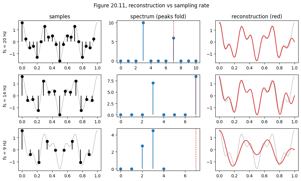
One band-limited signal (a sum of a 3 Hz and 7 Hz cosine, so $f_{\max}=7$) is sampled at
three rates. **Left:** the samples on the signal. **Middle:** the magnitude spectrum of
the samples: peaks land at the true frequencies only while Nyquist holds, otherwise they
fold. **Right:** sinc reconstruction (red) vs the original. Above Nyquist
($f_s>14$) it is exact; below, it is wrong.
```python theme={null}
# Band-limited test signal x(t) = cos(2 pi 3 t) + 0.6 cos(2 pi 7 t), f_max = 7 Hz.
def x_of(t):
return torch.cos(2 * math.pi * 3 * t) + 0.6 * torch.cos(2 * math.pi * 7 * t)
x_dense = x_of(t_cont)
rates = [20.0, 14.0, 9.0] # above Nyquist, at Nyquist, below (aliased)
recons, specs, sample_sets = [], [], []
for fr in rates:
tn = torch.arange(0, 1, 1.0 / fr, device=DEVICE)
xn = x_of(tn)
# sinc reconstruction from these samples onto the dense grid
r = (xn[:, None] * torch.sinc((t_cont[None, :] - tn[:, None]) * fr)).sum(0)
# magnitude spectrum of the sample sequence
mag = torch.fft.rfft(xn).abs()
freqs = torch.fft.rfftfreq(xn.numel(), d=1.0 / fr)
recons.append(r); specs.append((freqs, mag)); sample_sets.append((tn, xn))
print(f"sampled at rates {rates} Hz (Nyquist = {2*7} Hz)")
```
```output theme={null}
sampled at rates [20.0, 14.0, 9.0] Hz (Nyquist = 14 Hz)
```
## Figure 20.11: reconstruction degrades with sampling rate
One band-limited signal (a sum of a 3 Hz and 7 Hz cosine, so $f_{\max}=7$) is sampled at
three rates. **Left:** the samples on the signal. **Middle:** the magnitude spectrum of
the samples: peaks land at the true frequencies only while Nyquist holds, otherwise they
fold. **Right:** sinc reconstruction (red) vs the original. Above Nyquist
($f_s>14$) it is exact; below, it is wrong.
```python theme={null}
# Band-limited test signal x(t) = cos(2 pi 3 t) + 0.6 cos(2 pi 7 t), f_max = 7 Hz.
def x_of(t):
return torch.cos(2 * math.pi * 3 * t) + 0.6 * torch.cos(2 * math.pi * 7 * t)
x_dense = x_of(t_cont)
rates = [20.0, 14.0, 9.0] # above Nyquist, at Nyquist, below (aliased)
recons, specs, sample_sets = [], [], []
for fr in rates:
tn = torch.arange(0, 1, 1.0 / fr, device=DEVICE)
xn = x_of(tn)
# sinc reconstruction from these samples onto the dense grid
r = (xn[:, None] * torch.sinc((t_cont[None, :] - tn[:, None]) * fr)).sum(0)
# magnitude spectrum of the sample sequence
mag = torch.fft.rfft(xn).abs()
freqs = torch.fft.rfftfreq(xn.numel(), d=1.0 / fr)
recons.append(r); specs.append((freqs, mag)); sample_sets.append((tn, xn))
print(f"sampled at rates {rates} Hz (Nyquist = {2*7} Hz)")
```
```output theme={null}
sampled at rates [20.0, 14.0, 9.0] Hz (Nyquist = 14 Hz)
```
 ## Figure 20.12: local interpolation kernels
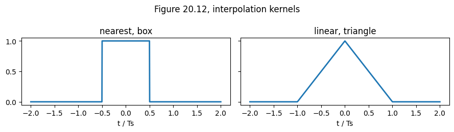
Ideal sinc reconstruction needs every sample. Cheaper *local* kernels trade accuracy for
support. **Nearest** interpolation convolves the samples with a box of width $T_s$;
**linear** interpolation convolves with a triangle of width $2T_s$ (the convolution of two
boxes). Both are shown as the kernel that the samples are convolved with.
```python theme={null}
# Nearest = box of width Ts; linear = triangle of width 2 Ts.
tk = torch.linspace(-2, 2, 1000, device=DEVICE)
box = torch.where(tk.abs() <= 0.5, torch.ones_like(tk), torch.zeros_like(tk))
triangle = torch.clamp(1 - tk.abs(), min=0.0)
print("nearest -> box kernel (width Ts) | linear -> triangle kernel (width 2 Ts)")
```
```output theme={null}
nearest -> box kernel (width Ts) | linear -> triangle kernel (width 2 Ts)
```
## Figure 20.12: local interpolation kernels
Ideal sinc reconstruction needs every sample. Cheaper *local* kernels trade accuracy for
support. **Nearest** interpolation convolves the samples with a box of width $T_s$;
**linear** interpolation convolves with a triangle of width $2T_s$ (the convolution of two
boxes). Both are shown as the kernel that the samples are convolved with.
```python theme={null}
# Nearest = box of width Ts; linear = triangle of width 2 Ts.
tk = torch.linspace(-2, 2, 1000, device=DEVICE)
box = torch.where(tk.abs() <= 0.5, torch.ones_like(tk), torch.zeros_like(tk))
triangle = torch.clamp(1 - tk.abs(), min=0.0)
print("nearest -> box kernel (width Ts) | linear -> triangle kernel (width 2 Ts)")
```
```output theme={null}
nearest -> box kernel (width Ts) | linear -> triangle kernel (width 2 Ts)
```
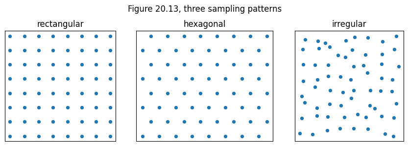
 ## Figure 20.13: 2-D sampling patterns
Images need not be sampled on a square grid. Three arrangements: a **rectangular** grid,
a **hexagonal** grid (alternate rows offset by half a step, rows spaced by
$\sqrt{3}/2$), and an **irregular** grid (jittered positions).
```python theme={null}
# Build rectangular, hexagonal, and irregular (jittered) sample positions.
n = 8
gx, gy = torch.meshgrid(torch.arange(n), torch.arange(n), indexing="ij")
rect = torch.stack([gx.flatten().float(), gy.flatten().float()], dim=1)
hex_pts = rect.clone()
hex_pts[:, 0] = hex_pts[:, 0] + 0.5 * (hex_pts[:, 1] % 2) # offset odd rows
hex_pts[:, 1] = hex_pts[:, 1] * (math.sqrt(3) / 2) # compress row spacing
irate = rect + 0.18 * torch.randn_like(rect) # jittered grid
print(f"{rect.shape[0]} points per pattern")
```
```output theme={null}
64 points per pattern
```
## Figure 20.13: 2-D sampling patterns
Images need not be sampled on a square grid. Three arrangements: a **rectangular** grid,
a **hexagonal** grid (alternate rows offset by half a step, rows spaced by
$\sqrt{3}/2$), and an **irregular** grid (jittered positions).
```python theme={null}
# Build rectangular, hexagonal, and irregular (jittered) sample positions.
n = 8
gx, gy = torch.meshgrid(torch.arange(n), torch.arange(n), indexing="ij")
rect = torch.stack([gx.flatten().float(), gy.flatten().float()], dim=1)
hex_pts = rect.clone()
hex_pts[:, 0] = hex_pts[:, 0] + 0.5 * (hex_pts[:, 1] % 2) # offset odd rows
hex_pts[:, 1] = hex_pts[:, 1] * (math.sqrt(3) / 2) # compress row spacing
irate = rect + 0.18 * torch.randn_like(rect) # jittered grid
print(f"{rect.shape[0]} points per pattern")
```
```output theme={null}
64 points per pattern
```
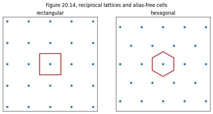
 ## Figure 20.14: Fourier transforms of the sampling lattices
In the frequency domain each sampling lattice repeats the spectrum on the **reciprocal
lattice**, and the no-aliasing region is its Voronoi cell (red). The rectangular lattice
gives a square cell; the hexagonal lattice gives a hexagon, which packs the largest
alias-free area per sample, about a 14% resolution gain.
```python theme={null}
# Reciprocal lattices and their Voronoi cells (the alias-free frequency region).
k = torch.arange(-2, 3)
ax_, ay_ = torch.meshgrid(k, k, indexing="ij")
rect_recip = torch.stack([ax_.flatten().float(), ay_.flatten().float()], dim=1)
hex_recip = rect_recip.clone() # reciprocal of a hex lattice
hex_recip[:, 0] = hex_recip[:, 0] + 0.5 * (hex_recip[:, 1] % 2)
hex_recip[:, 1] = hex_recip[:, 1] * (math.sqrt(3) / 2)
square_cell = torch.tensor([[-.5, -.5], [.5, -.5], [.5, .5], [-.5, .5], [-.5, -.5]])
ang = torch.linspace(0, 2 * math.pi, 7) # hexagon Voronoi cell
hexa = torch.stack([0.58 * torch.cos(ang + math.pi / 6), 0.58 * torch.sin(ang + math.pi / 6)], 1)
print("rect cell: square | hex cell: hexagon (larger alias-free area)")
```
```output theme={null}
rect cell: square | hex cell: hexagon (larger alias-free area)
```
## Figure 20.14: Fourier transforms of the sampling lattices
In the frequency domain each sampling lattice repeats the spectrum on the **reciprocal
lattice**, and the no-aliasing region is its Voronoi cell (red). The rectangular lattice
gives a square cell; the hexagonal lattice gives a hexagon, which packs the largest
alias-free area per sample, about a 14% resolution gain.
```python theme={null}
# Reciprocal lattices and their Voronoi cells (the alias-free frequency region).
k = torch.arange(-2, 3)
ax_, ay_ = torch.meshgrid(k, k, indexing="ij")
rect_recip = torch.stack([ax_.flatten().float(), ay_.flatten().float()], dim=1)
hex_recip = rect_recip.clone() # reciprocal of a hex lattice
hex_recip[:, 0] = hex_recip[:, 0] + 0.5 * (hex_recip[:, 1] % 2)
hex_recip[:, 1] = hex_recip[:, 1] * (math.sqrt(3) / 2)
square_cell = torch.tensor([[-.5, -.5], [.5, -.5], [.5, .5], [-.5, .5], [-.5, -.5]])
ang = torch.linspace(0, 2 * math.pi, 7) # hexagon Voronoi cell
hexa = torch.stack([0.58 * torch.cos(ang + math.pi / 6), 0.58 * torch.sin(ang + math.pi / 6)], 1)
print("rect cell: square | hex cell: hexagon (larger alias-free area)")
```
```output theme={null}
rect cell: square | hex cell: hexagon (larger alias-free area)
```
 ## Figure 20.15: the cone mosaic
The book illustrates that the photoreceptors in the primate fovea sit on an approximately hexagonal lattice, using a micrograph of a monkey retina from Curcio et al. ([Figure 20.15](https://visionbook.mit.edu/sampling_and_aliasing.html#fig-samplingfovea)). That is measured microscopy, not a computed plot, so there is nothing to regenerate here. The previous figure already shows *why* hexagonal sampling is favored.
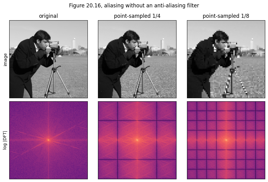
## Figure 20.16: aliasing in a real image
The book downsamples a [photograph of a zebra](https://visionbook.mit.edu/sampling_and_aliasing.html#fig-aliasingFTzebra) and the stripes change orientation. Here the public-domain *cameraman* test image stands in for it: you **point-sample** it with no pre-filter at two rates. Reconstructed to full size, the fine detail (tripod, coat texture) breaks up, and the log magnitude spectrum shows energy folding inward.
```python theme={null}
# Load the cameraman test image as a single-channel float tensor in [0, 1].
# stand-in for a photograph of a zebra in the book; original: https://visionbook.mit.edu/sampling_and_aliasing.html#fig-aliasingFTzebra
img = (torch.from_numpy(camera().copy()).float() / 255.0).to(DEVICE)
def point_sample(x, s):
# keep every s-th pixel (no pre-filter), then nearest-upscale to full size for comparison
ds = x[::s, ::s]
return ds.repeat_interleave(s, 0).repeat_interleave(s, 1)[: x.shape[0], : x.shape[1]]
def log_spectrum(x):
return torch.fft.fftshift(torch.fft.fft2(x)).abs().add(1e-3).log()
aliased_4 = point_sample(img, 4)
aliased_8 = point_sample(img, 8)
print(f"image {tuple(img.shape)} point-sampled at 1/4 and 1/8")
```
```output theme={null}
image (512, 512) point-sampled at 1/4 and 1/8
```
## Figure 20.15: the cone mosaic
The book illustrates that the photoreceptors in the primate fovea sit on an approximately hexagonal lattice, using a micrograph of a monkey retina from Curcio et al. ([Figure 20.15](https://visionbook.mit.edu/sampling_and_aliasing.html#fig-samplingfovea)). That is measured microscopy, not a computed plot, so there is nothing to regenerate here. The previous figure already shows *why* hexagonal sampling is favored.
## Figure 20.16: aliasing in a real image
The book downsamples a [photograph of a zebra](https://visionbook.mit.edu/sampling_and_aliasing.html#fig-aliasingFTzebra) and the stripes change orientation. Here the public-domain *cameraman* test image stands in for it: you **point-sample** it with no pre-filter at two rates. Reconstructed to full size, the fine detail (tripod, coat texture) breaks up, and the log magnitude spectrum shows energy folding inward.
```python theme={null}
# Load the cameraman test image as a single-channel float tensor in [0, 1].
# stand-in for a photograph of a zebra in the book; original: https://visionbook.mit.edu/sampling_and_aliasing.html#fig-aliasingFTzebra
img = (torch.from_numpy(camera().copy()).float() / 255.0).to(DEVICE)
def point_sample(x, s):
# keep every s-th pixel (no pre-filter), then nearest-upscale to full size for comparison
ds = x[::s, ::s]
return ds.repeat_interleave(s, 0).repeat_interleave(s, 1)[: x.shape[0], : x.shape[1]]
def log_spectrum(x):
return torch.fft.fftshift(torch.fft.fft2(x)).abs().add(1e-3).log()
aliased_4 = point_sample(img, 4)
aliased_8 = point_sample(img, 8)
print(f"image {tuple(img.shape)} point-sampled at 1/4 and 1/8")
```
```output theme={null}
image (512, 512) point-sampled at 1/4 and 1/8
```
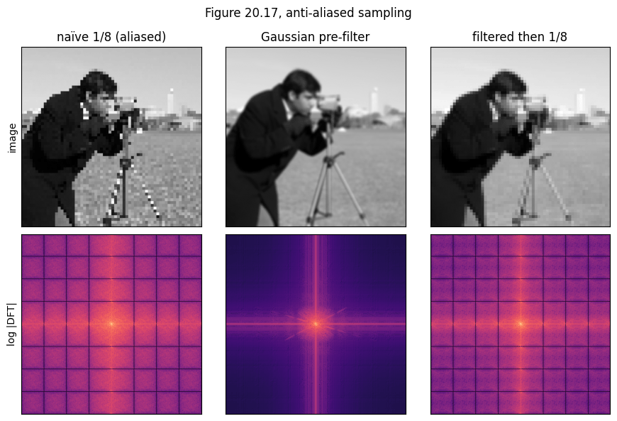
 ## Figure 20.17: the anti-aliasing filter
Blurring with a low-pass filter *before* sampling removes the frequencies the grid cannot represent, so they no longer fold. The next cell applies a Kornia Gaussian blur, then point-samples at the same 1/8 rate. The result keeps the recognizable low-frequency structure, and its spectrum no longer shows the aliased fold-in, at the cost of the lost (genuinely unrepresentable) detail.
```python theme={null}
# Anti-alias: Gaussian low-pass (Kornia) BEFORE point-sampling, vs the naive 1/8 above.
def blur(x, ksize, sigma):
out = kornia.filters.gaussian_blur2d(x[None, None], (ksize, ksize), (sigma, sigma))
return out[0, 0]
prefiltered = blur(img, 11, 4.0)
antialiased_8 = point_sample(prefiltered, 8)
print("Gaussian pre-filter (sigma=4) applied before 1/8 sampling")
```
```output theme={null}
Gaussian pre-filter (sigma=4) applied before 1/8 sampling
```
## Figure 20.17: the anti-aliasing filter
Blurring with a low-pass filter *before* sampling removes the frequencies the grid cannot represent, so they no longer fold. The next cell applies a Kornia Gaussian blur, then point-samples at the same 1/8 rate. The result keeps the recognizable low-frequency structure, and its spectrum no longer shows the aliased fold-in, at the cost of the lost (genuinely unrepresentable) detail.
```python theme={null}
# Anti-alias: Gaussian low-pass (Kornia) BEFORE point-sampling, vs the naive 1/8 above.
def blur(x, ksize, sigma):
out = kornia.filters.gaussian_blur2d(x[None, None], (ksize, ksize), (sigma, sigma))
return out[0, 0]
prefiltered = blur(img, 11, 4.0)
antialiased_8 = point_sample(prefiltered, 8)
print("Gaussian pre-filter (sigma=4) applied before 1/8 sampling")
```
```output theme={null}
Gaussian pre-filter (sigma=4) applied before 1/8 sampling
```
 ## Concluding remarks
Aliasing appears whenever a continuous light field is sampled, and again at every
downsampling or upsampling step (chapter 21 of the book). The sampling theorem says it is avoided when
$f_s > 2 f_{\max}$; when it cannot be (a finite-resolution grid is never band-limited), an
anti-aliasing filter trades unrepresentable detail for an artifact-free image. Aliasing is
not always harmful: super-resolution methods exploit it to recover detail across frames.
**Reference.** A. Torralba, P. Isola, W. T. Freeman, *Foundations of Computer Vision*,
MIT Press, chapter 20, [visionbook.mit.edu](https://visionbook.mit.edu/sampling_and_aliasing.html).
***
[Edit this page on GitHub](https://github.com/aegean-ai/eaia/edit/main/src/aiml-common/lectures/image-processing/sampling-and-aliasing/index.mdx) or [file an issue](https://github.com/aegean-ai/eaia/issues/new/choose).
## Concluding remarks
Aliasing appears whenever a continuous light field is sampled, and again at every
downsampling or upsampling step (chapter 21 of the book). The sampling theorem says it is avoided when
$f_s > 2 f_{\max}$; when it cannot be (a finite-resolution grid is never band-limited), an
anti-aliasing filter trades unrepresentable detail for an artifact-free image. Aliasing is
not always harmful: super-resolution methods exploit it to recover detail across frames.
**Reference.** A. Torralba, P. Isola, W. T. Freeman, *Foundations of Computer Vision*,
MIT Press, chapter 20, [visionbook.mit.edu](https://visionbook.mit.edu/sampling_and_aliasing.html).
***
[Edit this page on GitHub](https://github.com/aegean-ai/eaia/edit/main/src/aiml-common/lectures/image-processing/sampling-and-aliasing/index.mdx) or [file an issue](https://github.com/aegean-ai/eaia/issues/new/choose).