> ## Documentation Index
> Fetch the complete documentation index at: https://aegean.ai/llms.txt
> Use this file to discover all available pages before exploring further.
# What Natural Images Have in Common
> The 1/f power law, correlated pixels, heavy-tailed derivatives, and how these priors drive Wiener filtering, coring, and non-local means.
 *This section was written by [Kaushik Kachireddy](https://github.com/kaushik0x7d2) ([pull request #79](https://github.com/pantelis/eng-ai-agents/pull/79)), with help from an AI coding agent (Claude Code) on the code. It reproduces the ideas of Chapter 27 of [*Foundations of Computer Vision*](https://visionbook.mit.edu/stat_image_models_revised.html) by Antonio Torralba, Phillip Isola, and William T. Freeman. The book's own figures are not reproduced here, because the book's license covers only the work in full; links point to them instead.*
Natural images are a **vanishingly small, highly structured** corner of the space of all pixel arrays. This section measures that structure and builds generative priors from it: the **1/f power law**, sampling clouds from it, why an independent-pixel model fails, the **decay of pixel correlations**, the **heavy-tailed (generalized-Laplacian) statistics of derivatives**, and how those priors drive **denoising**: Wiener filtering, wavelet **coring**, and **non-local means**.
The book measures these statistics on its own photographs. Here the measurements run on scikit-image test photographs (an astronaut, a rocket, a coffee cup, the cameraman, a cat, a clock, grass, and a Hubble deep field) and on generated images, and each figure links to the book's version. The statistics are properties of natural images in general, so they come out the same.
```python theme={null}
import numpy as np
import matplotlib.pyplot as plt
from scipy.special import gamma
from skimage.color import rgb2gray
from skimage.transform import resize
np.random.seed(0)
plt.rcParams.update({'figure.dpi': 130, 'savefig.dpi': 130,
'image.cmap': 'gray', 'axes.grid': False})
```
**Images replaced for licensing.** The book is published under a CC BY-NC-ND license, which covers only the book as a whole and not its individual images, so this page does not republish the book's photographs. License-free images stand in for them:
* The *astronaut*, *rocket*, and *coffee* photographs (scikit-image) stand in for [photographs of the MIT dome, a wheel, and autumn leaves (Figure 27.10)](https://visionbook.mit.edu/stat_image_models_revised.html#fig-FT_angular_averages).
* The *cameraman* photograph (scikit-image) stands in for [a photograph of a street (Figures 27.8 and 27.15)](https://visionbook.mit.edu/stat_image_models_revised.html#fig-correlation).
* The *chelsea* photograph (scikit-image) stands in for [a photograph of colorful houses (Figure 27.23)](https://visionbook.mit.edu/stat_image_models_revised.html#fig-nlm2).
* The *clock* photograph (scikit-image) stands in for [a photograph of a doorway (Figure 27.16)](https://visionbook.mit.edu/stat_image_models_revised.html#fig-derivativesdistributions).
* The *grass* texture (scikit-image) stands in for [a photograph of hair (Figure 27.13)](https://visionbook.mit.edu/stat_image_models_revised.html#fig-hair).
* The *cameraman* photograph (scikit-image) stands in for [a photograph of a building in Barcelona (Figure 27.14)](https://visionbook.mit.edu/stat_image_models_revised.html#fig-denoisingGaussianModel).
* The Hubble deep field, *immunohistochemistry*, and *colorwheel* images (scikit-image) and generated clouds stand in for [photographs of stars, clouds, plums, and a cube (Figures 27.6 and 27.12)](https://visionbook.mit.edu/stat_image_models_revised.html#fig-histMatch).
* Generated images and scikit-image photographs stand in for [the book's eight visual worlds (Figure 27.2)](https://visionbook.mit.edu/stat_image_models_revised.html#fig-worlds).
If you use the book for non-commercial purposes, you can swap the originals back in: each line that loads a stand-in carries the original's link in a comment.
```python theme={null}
def to_gray_square(img, size=256):
"""Grayscale, center-crop to square, resize to size x size, in [0,1]."""
g = rgb2gray(img) if img.ndim == 3 else img
h, w = g.shape; s = min(h, w)
g = g[(h - s) // 2:(h - s) // 2 + s, (w - s) // 2:(w - s) // 2 + s]
return resize(g, (size, size), anti_aliasing=True)
def radial_profile(mag):
"""Angular-averaged radial profile of a 2D (fft-shifted) magnitude image."""
h, w = mag.shape; cy, cx = h // 2, w // 2
y, x = np.indices((h, w))
r = np.sqrt((x - cx)**2 + (y - cy)**2).astype(int)
tbin = np.bincount(r.ravel(), mag.ravel())
nr = np.bincount(r.ravel())
return tbin / np.maximum(nr, 1)
def gen_laplacian(x, r, s=1.0):
"""Generalized Laplacian pdf exp(-|x/s|^r) / (2 (s/r) Gamma(1/r))."""
return np.exp(-np.abs(x / s)**r) / (2 * (s / r) * gamma(1.0 / r))
```
```python theme={null}
def _kurt(a):
a = a - a.mean(); return float((a**4).mean() / (a.var()**2 + 1e-12))
```
```python theme={null}
from skimage import data, img_as_float
def rgbf(im):
"""float RGB in [0, 1] from a scikit-image array (grayscale is repeated over 3 channels)."""
im = img_as_float(im).astype(np.float32)
return np.repeat(im[..., None], 3, -1) if im.ndim == 2 else im[..., :3]
def clouds(size=256, alpha=1.5, seed=0):
"""Color 1/f noise: a random-phase sample per channel (the 'clouds' of 27.11)."""
g = np.random.default_rng(seed); fy = np.fft.fftfreq(size)[:, None]; fx = np.fft.fftfreq(size)[None, :]
mag = 1.0 / (1.0 + (size * np.sqrt(fx**2 + fy**2))**alpha)
out = np.stack([np.real(np.fft.ifft2(mag * np.exp(2j * np.pi * g.random((size, size))))) for _ in range(3)], -1)
return (out - out.min()) / (np.ptp(out) + 1e-9)
# Test photographs in place of the book's images (see the links next to each figure)
# stand-in for photographs of the MIT dome, a wheel, and autumn leaves in the book; original: https://visionbook.mit.edu/stat_image_models_revised.html#fig-FT_angular_averages
DOME, WHEEL, LEAVES = rgbf(data.astronaut()), rgbf(data.rocket()), rgbf(data.coffee()) # 27.10
# stand-in for a photograph of a street in the book; original: https://visionbook.mit.edu/stat_image_models_revised.html#fig-correlation
STREET = rgbf(data.camera()) # grayscale scene (27.8, 27.15)
# stand-in for a photograph of colorful houses in the book; original: https://visionbook.mit.edu/stat_image_models_revised.html#fig-nlm2
BURANO = rgbf(data.chelsea()) # color scene for non-local means (27.23)
# stand-in for a photograph of a doorway in the book; original: https://visionbook.mit.edu/stat_image_models_revised.html#fig-derivativesdistributions
BUILDING = rgbf(data.clock()) # grayscale object photo (27.16)
# stand-in for a photograph of hair in the book; original: https://visionbook.mit.edu/stat_image_models_revised.html#fig-hair
HAIR = rgbf(data.grass()) # oriented texture, in place of hair (27.13, 27.16)
# stand-in for a photograph of a building in Barcelona in the book; original: https://visionbook.mit.edu/stat_image_models_revised.html#fig-denoisingGaussianModel
BCN = rgbf(data.camera()) # grayscale scene for Wiener denoising (27.14)
# stand-in for photographs of stars, clouds, plums, and a cube in the book; original: https://visionbook.mit.edu/stat_image_models_revised.html#fig-histMatch
STARS = rgbf(data.hubble_deep_field())[:400, :400] # a real star field (27.6, 27.12)
CLOUDS = clouds() # generated clouds (27.6, 27.12)
PLUMS = rgbf(data.immunohistochemistry()) # blob-like color image (27.6, 27.12)
CUBE = rgbf(data.colorwheel()) # smooth color structure (27.6, 27.12)
print('street', STREET.shape, ' stars', STARS.shape, ' clouds', CLOUDS.shape)
```
```output theme={null}
street (512, 512, 3) stars (400, 400, 3) clouds (256, 256, 3)
```
## The 1/f power law
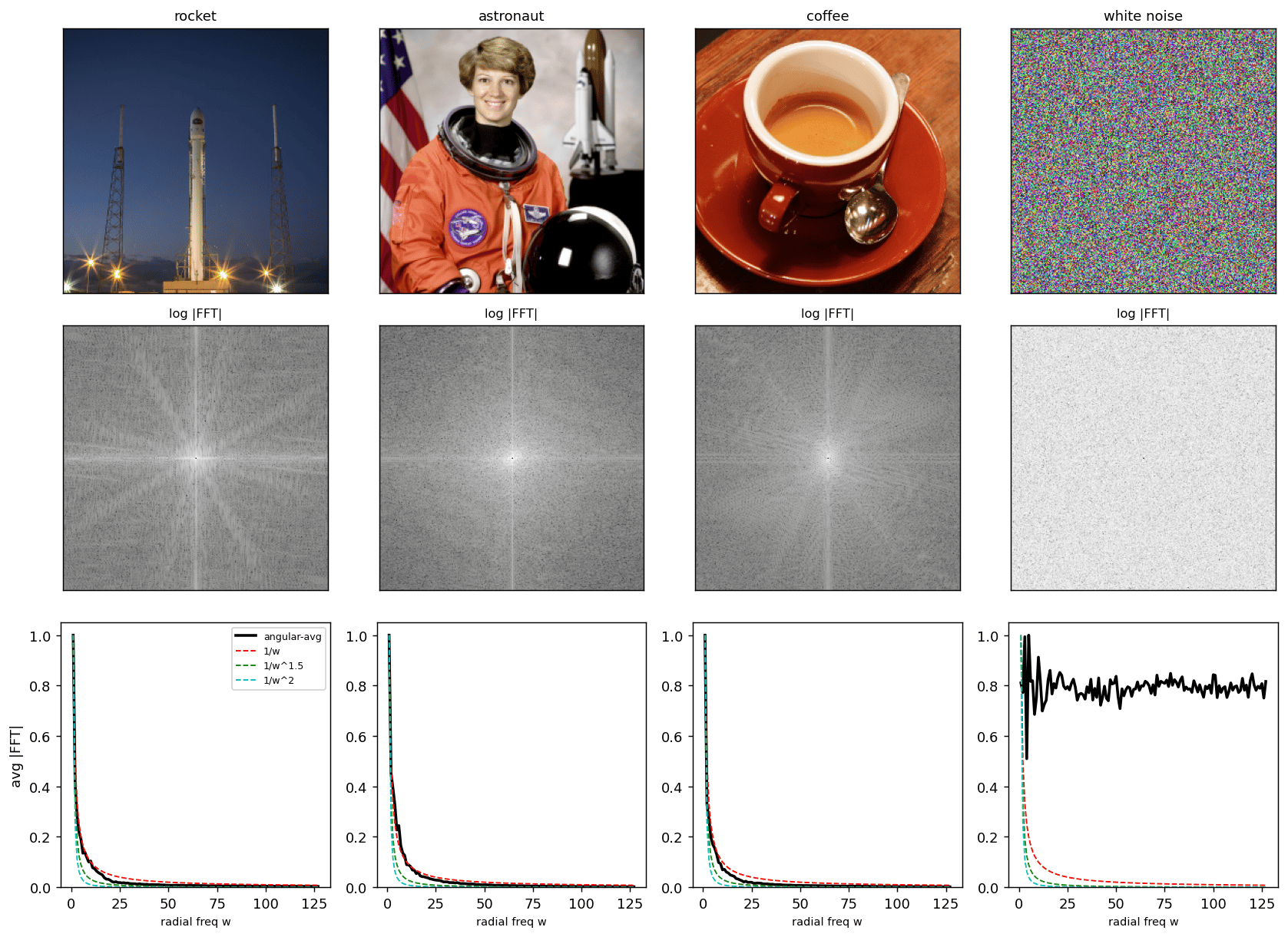
The single most robust statistic of natural images: the Fourier magnitude falls off as a **power law** in radial frequency,
$\lVert\mathscr L(u,v)\rVert \;\simeq\; \frac{1}{w^{\alpha}},\qquad w=\sqrt{u^2+v^2},\ \ \alpha\approx 1\text{ to }1.5.$
Three real photos concentrate their energy (the book's version is [Figure 27.10](https://visionbook.mit.edu/stat_image_models_revised.html#fig-FT_angular_averages)) at low frequency and their angular-averaged spectra hug the $1/w^{1.5}$ curve; **white noise is flat**: no power law at all.
```python theme={null}
# Figure 27.10: images (top, COLOR as in the book), |FFT| (mid), radial spectra (bottom).
def sq_col(img, size=256):
h, w = img.shape[:2]; s = min(h, w)
c = img[(h - s) // 2:(h - s) // 2 + s, (w - s) // 2:(w - s) // 2 + s]
return resize(c, (size, size), anti_aliasing=True)
noise_rgb = np.random.rand(256, 256, 3) # color white noise (book uses RGB)
imgs = [('rocket', sq_col(WHEEL)), ('astronaut', sq_col(DOME)),
('coffee', sq_col(LEAVES)), ('white noise', noise_rgb)]
```
*This section was written by [Kaushik Kachireddy](https://github.com/kaushik0x7d2) ([pull request #79](https://github.com/pantelis/eng-ai-agents/pull/79)), with help from an AI coding agent (Claude Code) on the code. It reproduces the ideas of Chapter 27 of [*Foundations of Computer Vision*](https://visionbook.mit.edu/stat_image_models_revised.html) by Antonio Torralba, Phillip Isola, and William T. Freeman. The book's own figures are not reproduced here, because the book's license covers only the work in full; links point to them instead.*
Natural images are a **vanishingly small, highly structured** corner of the space of all pixel arrays. This section measures that structure and builds generative priors from it: the **1/f power law**, sampling clouds from it, why an independent-pixel model fails, the **decay of pixel correlations**, the **heavy-tailed (generalized-Laplacian) statistics of derivatives**, and how those priors drive **denoising**: Wiener filtering, wavelet **coring**, and **non-local means**.
The book measures these statistics on its own photographs. Here the measurements run on scikit-image test photographs (an astronaut, a rocket, a coffee cup, the cameraman, a cat, a clock, grass, and a Hubble deep field) and on generated images, and each figure links to the book's version. The statistics are properties of natural images in general, so they come out the same.
```python theme={null}
import numpy as np
import matplotlib.pyplot as plt
from scipy.special import gamma
from skimage.color import rgb2gray
from skimage.transform import resize
np.random.seed(0)
plt.rcParams.update({'figure.dpi': 130, 'savefig.dpi': 130,
'image.cmap': 'gray', 'axes.grid': False})
```
**Images replaced for licensing.** The book is published under a CC BY-NC-ND license, which covers only the book as a whole and not its individual images, so this page does not republish the book's photographs. License-free images stand in for them:
* The *astronaut*, *rocket*, and *coffee* photographs (scikit-image) stand in for [photographs of the MIT dome, a wheel, and autumn leaves (Figure 27.10)](https://visionbook.mit.edu/stat_image_models_revised.html#fig-FT_angular_averages).
* The *cameraman* photograph (scikit-image) stands in for [a photograph of a street (Figures 27.8 and 27.15)](https://visionbook.mit.edu/stat_image_models_revised.html#fig-correlation).
* The *chelsea* photograph (scikit-image) stands in for [a photograph of colorful houses (Figure 27.23)](https://visionbook.mit.edu/stat_image_models_revised.html#fig-nlm2).
* The *clock* photograph (scikit-image) stands in for [a photograph of a doorway (Figure 27.16)](https://visionbook.mit.edu/stat_image_models_revised.html#fig-derivativesdistributions).
* The *grass* texture (scikit-image) stands in for [a photograph of hair (Figure 27.13)](https://visionbook.mit.edu/stat_image_models_revised.html#fig-hair).
* The *cameraman* photograph (scikit-image) stands in for [a photograph of a building in Barcelona (Figure 27.14)](https://visionbook.mit.edu/stat_image_models_revised.html#fig-denoisingGaussianModel).
* The Hubble deep field, *immunohistochemistry*, and *colorwheel* images (scikit-image) and generated clouds stand in for [photographs of stars, clouds, plums, and a cube (Figures 27.6 and 27.12)](https://visionbook.mit.edu/stat_image_models_revised.html#fig-histMatch).
* Generated images and scikit-image photographs stand in for [the book's eight visual worlds (Figure 27.2)](https://visionbook.mit.edu/stat_image_models_revised.html#fig-worlds).
If you use the book for non-commercial purposes, you can swap the originals back in: each line that loads a stand-in carries the original's link in a comment.
```python theme={null}
def to_gray_square(img, size=256):
"""Grayscale, center-crop to square, resize to size x size, in [0,1]."""
g = rgb2gray(img) if img.ndim == 3 else img
h, w = g.shape; s = min(h, w)
g = g[(h - s) // 2:(h - s) // 2 + s, (w - s) // 2:(w - s) // 2 + s]
return resize(g, (size, size), anti_aliasing=True)
def radial_profile(mag):
"""Angular-averaged radial profile of a 2D (fft-shifted) magnitude image."""
h, w = mag.shape; cy, cx = h // 2, w // 2
y, x = np.indices((h, w))
r = np.sqrt((x - cx)**2 + (y - cy)**2).astype(int)
tbin = np.bincount(r.ravel(), mag.ravel())
nr = np.bincount(r.ravel())
return tbin / np.maximum(nr, 1)
def gen_laplacian(x, r, s=1.0):
"""Generalized Laplacian pdf exp(-|x/s|^r) / (2 (s/r) Gamma(1/r))."""
return np.exp(-np.abs(x / s)**r) / (2 * (s / r) * gamma(1.0 / r))
```
```python theme={null}
def _kurt(a):
a = a - a.mean(); return float((a**4).mean() / (a.var()**2 + 1e-12))
```
```python theme={null}
from skimage import data, img_as_float
def rgbf(im):
"""float RGB in [0, 1] from a scikit-image array (grayscale is repeated over 3 channels)."""
im = img_as_float(im).astype(np.float32)
return np.repeat(im[..., None], 3, -1) if im.ndim == 2 else im[..., :3]
def clouds(size=256, alpha=1.5, seed=0):
"""Color 1/f noise: a random-phase sample per channel (the 'clouds' of 27.11)."""
g = np.random.default_rng(seed); fy = np.fft.fftfreq(size)[:, None]; fx = np.fft.fftfreq(size)[None, :]
mag = 1.0 / (1.0 + (size * np.sqrt(fx**2 + fy**2))**alpha)
out = np.stack([np.real(np.fft.ifft2(mag * np.exp(2j * np.pi * g.random((size, size))))) for _ in range(3)], -1)
return (out - out.min()) / (np.ptp(out) + 1e-9)
# Test photographs in place of the book's images (see the links next to each figure)
# stand-in for photographs of the MIT dome, a wheel, and autumn leaves in the book; original: https://visionbook.mit.edu/stat_image_models_revised.html#fig-FT_angular_averages
DOME, WHEEL, LEAVES = rgbf(data.astronaut()), rgbf(data.rocket()), rgbf(data.coffee()) # 27.10
# stand-in for a photograph of a street in the book; original: https://visionbook.mit.edu/stat_image_models_revised.html#fig-correlation
STREET = rgbf(data.camera()) # grayscale scene (27.8, 27.15)
# stand-in for a photograph of colorful houses in the book; original: https://visionbook.mit.edu/stat_image_models_revised.html#fig-nlm2
BURANO = rgbf(data.chelsea()) # color scene for non-local means (27.23)
# stand-in for a photograph of a doorway in the book; original: https://visionbook.mit.edu/stat_image_models_revised.html#fig-derivativesdistributions
BUILDING = rgbf(data.clock()) # grayscale object photo (27.16)
# stand-in for a photograph of hair in the book; original: https://visionbook.mit.edu/stat_image_models_revised.html#fig-hair
HAIR = rgbf(data.grass()) # oriented texture, in place of hair (27.13, 27.16)
# stand-in for a photograph of a building in Barcelona in the book; original: https://visionbook.mit.edu/stat_image_models_revised.html#fig-denoisingGaussianModel
BCN = rgbf(data.camera()) # grayscale scene for Wiener denoising (27.14)
# stand-in for photographs of stars, clouds, plums, and a cube in the book; original: https://visionbook.mit.edu/stat_image_models_revised.html#fig-histMatch
STARS = rgbf(data.hubble_deep_field())[:400, :400] # a real star field (27.6, 27.12)
CLOUDS = clouds() # generated clouds (27.6, 27.12)
PLUMS = rgbf(data.immunohistochemistry()) # blob-like color image (27.6, 27.12)
CUBE = rgbf(data.colorwheel()) # smooth color structure (27.6, 27.12)
print('street', STREET.shape, ' stars', STARS.shape, ' clouds', CLOUDS.shape)
```
```output theme={null}
street (512, 512, 3) stars (400, 400, 3) clouds (256, 256, 3)
```
## The 1/f power law
The single most robust statistic of natural images: the Fourier magnitude falls off as a **power law** in radial frequency,
$\lVert\mathscr L(u,v)\rVert \;\simeq\; \frac{1}{w^{\alpha}},\qquad w=\sqrt{u^2+v^2},\ \ \alpha\approx 1\text{ to }1.5.$
Three real photos concentrate their energy (the book's version is [Figure 27.10](https://visionbook.mit.edu/stat_image_models_revised.html#fig-FT_angular_averages)) at low frequency and their angular-averaged spectra hug the $1/w^{1.5}$ curve; **white noise is flat**: no power law at all.
```python theme={null}
# Figure 27.10: images (top, COLOR as in the book), |FFT| (mid), radial spectra (bottom).
def sq_col(img, size=256):
h, w = img.shape[:2]; s = min(h, w)
c = img[(h - s) // 2:(h - s) // 2 + s, (w - s) // 2:(w - s) // 2 + s]
return resize(c, (size, size), anti_aliasing=True)
noise_rgb = np.random.rand(256, 256, 3) # color white noise (book uses RGB)
imgs = [('rocket', sq_col(WHEEL)), ('astronaut', sq_col(DOME)),
('coffee', sq_col(LEAVES)), ('white noise', noise_rgb)]
```
 ## Sampling from the power spectrum
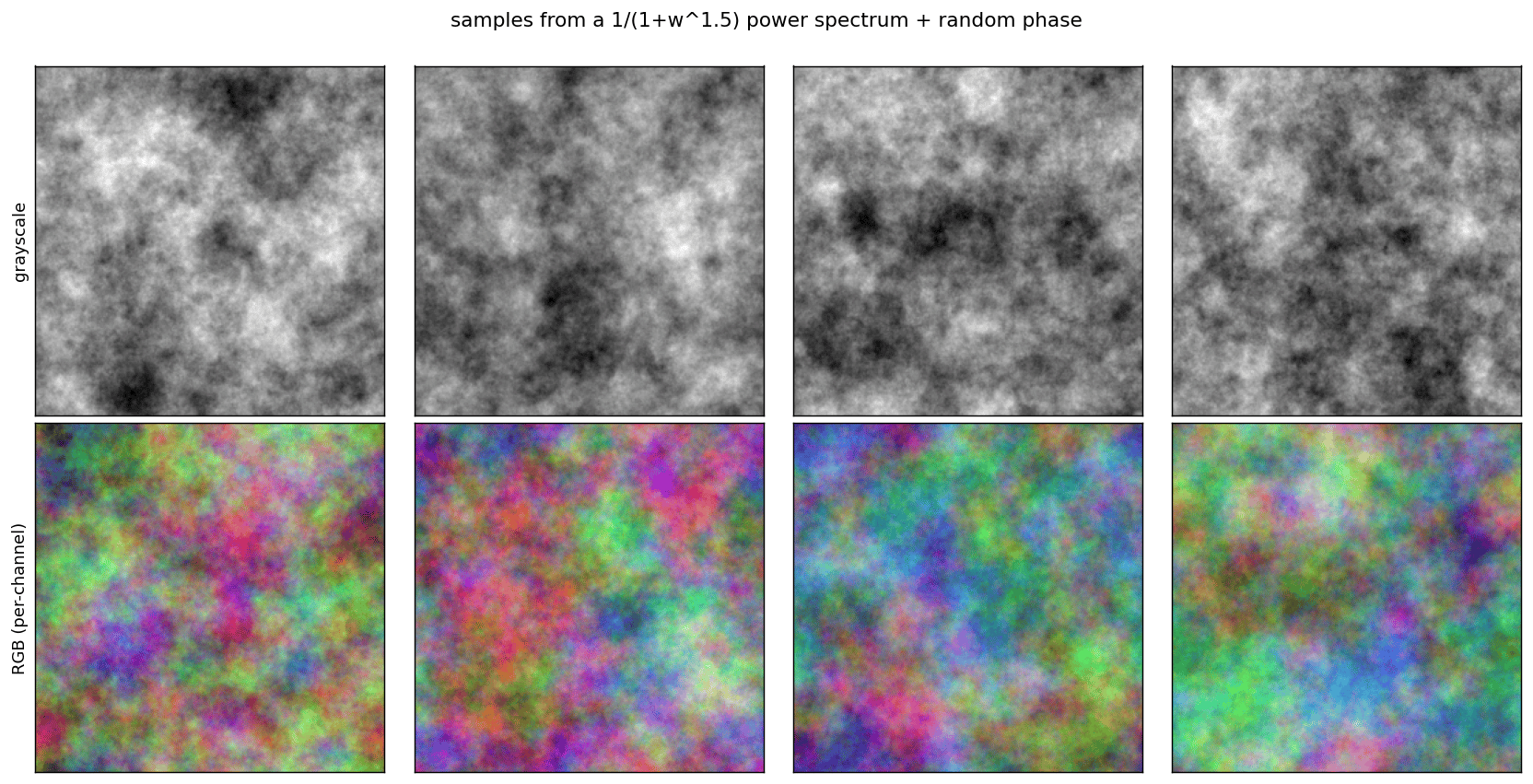
A Gaussian image prior with a $1/(1+w^{\alpha})$ power spectrum is easy to sample: take that magnitude, attach **random phase**, and inverse-transform. The result has the right spectral falloff but no real structure: it always looks like **clouds**, in grayscale or (sampling each channel) in color.
```python theme={null}
# Figure 27.11: cloud samples from a 1/(1+w^1.5) spectrum, gray (top) + RGB (bottom).
def one_over_f_sample(size=256, alpha=1.5, rng=None):
rng = rng or np.random
fy = np.fft.fftfreq(size)[:, None]; fx = np.fft.fftfreq(size)[None, :]
w = np.sqrt(fx**2 + fy**2); mag = 1.0 / (1.0 + (size * w)**alpha)
phase = np.exp(2j * np.pi * rng.rand(size, size))
img = np.real(np.fft.ifft2(mag * phase))
return (img - img.min()) / (np.ptp(img) + 1e-9)
```
## Sampling from the power spectrum
A Gaussian image prior with a $1/(1+w^{\alpha})$ power spectrum is easy to sample: take that magnitude, attach **random phase**, and inverse-transform. The result has the right spectral falloff but no real structure: it always looks like **clouds**, in grayscale or (sampling each channel) in color.
```python theme={null}
# Figure 27.11: cloud samples from a 1/(1+w^1.5) spectrum, gray (top) + RGB (bottom).
def one_over_f_sample(size=256, alpha=1.5, rng=None):
rng = rng or np.random
fy = np.fft.fftfreq(size)[:, None]; fx = np.fft.fftfreq(size)[None, :]
w = np.sqrt(fx**2 + fy**2); mag = 1.0 / (1.0 + (size * w)**alpha)
phase = np.exp(2j * np.pi * rng.rand(size, size))
img = np.real(np.fft.ifft2(mag * phase))
return (img - img.min()) / (np.ptp(img) + 1e-9)
```
 ## The independent-pixel model
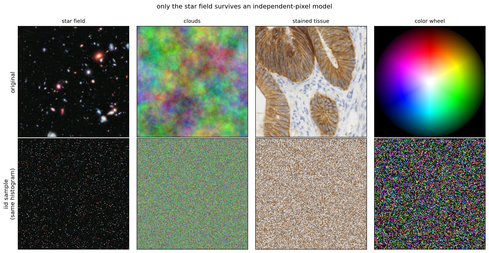
The simplest model treats every pixel as an independent draw from one histogram. Sampling from it keeps the image's **color and intensity distribution** exactly but destroys all spatial arrangement: the sample is just noise with the right histogram. It only ever looks right for images that *are* essentially unstructured, like a star field. The book's version is [Figure 27.6](https://visionbook.mit.edu/stat_image_models_revised.html#fig-histMatch).
```python theme={null}
# Figure 27.6: original (top) vs independent-pixel sample (bottom), four
# images. An iid draw from the exact color histogram = a random shuffle of
# the pixels: same histogram, all structure gone.
def iid_sample(img):
flat = img.reshape(-1, img.shape[-1])
return flat[np.random.permutation(len(flat))].reshape(img.shape)
def sq(img, size=200):
h, w = img.shape[:2]; s = min(h, w)
return resize(img[(h - s) // 2:(h - s) // 2 + s, (w - s) // 2:(w - s) // 2 + s],
(size, size), anti_aliasing=True)
pics = [('star field', sq(STARS)), ('clouds', sq(CLOUDS)),
('stained tissue', sq(PLUMS)), ('color wheel', sq(CUBE))]
```
## The independent-pixel model
The simplest model treats every pixel as an independent draw from one histogram. Sampling from it keeps the image's **color and intensity distribution** exactly but destroys all spatial arrangement: the sample is just noise with the right histogram. It only ever looks right for images that *are* essentially unstructured, like a star field. The book's version is [Figure 27.6](https://visionbook.mit.edu/stat_image_models_revised.html#fig-histMatch).
```python theme={null}
# Figure 27.6: original (top) vs independent-pixel sample (bottom), four
# images. An iid draw from the exact color histogram = a random shuffle of
# the pixels: same histogram, all structure gone.
def iid_sample(img):
flat = img.reshape(-1, img.shape[-1])
return flat[np.random.permutation(len(flat))].reshape(img.shape)
def sq(img, size=200):
h, w = img.shape[:2]; s = min(h, w)
return resize(img[(h - s) // 2:(h - s) // 2 + s, (w - s) // 2:(w - s) // 2 + s],
(size, size), anti_aliasing=True)
pics = [('star field', sq(STARS)), ('clouds', sq(CLOUDS)),
('stained tissue', sq(PLUMS)), ('color wheel', sq(CUBE))]
```
 ## Pixel correlations decay with distance
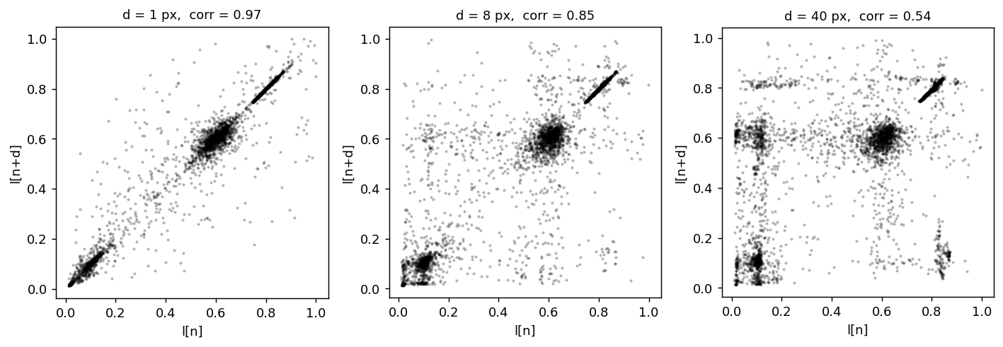
Neighboring pixels are highly correlated; the correlation falls as they move apart. Scatter plots of $\ell[n]$ vs $\ell[n+d]$ tighten around the diagonal for small $d$ and spread out for large $d$ (the book's version is [Figure 27.8](https://visionbook.mit.edu/stat_image_models_revised.html#fig-correlation)).
```python theme={null}
# Figure 27.8: pixel-pair scatter at increasing horizontal distance d.
g = to_gray_square(STREET, 256)
```
## Pixel correlations decay with distance
Neighboring pixels are highly correlated; the correlation falls as they move apart. Scatter plots of $\ell[n]$ vs $\ell[n+d]$ tighten around the diagonal for small $d$ and spread out for large $d$ (the book's version is [Figure 27.8](https://visionbook.mit.edu/stat_image_models_revised.html#fig-correlation)).
```python theme={null}
# Figure 27.8: pixel-pair scatter at increasing horizontal distance d.
g = to_gray_square(STREET, 256)
```
 ## Derivatives are heavy-tailed, not Gaussian
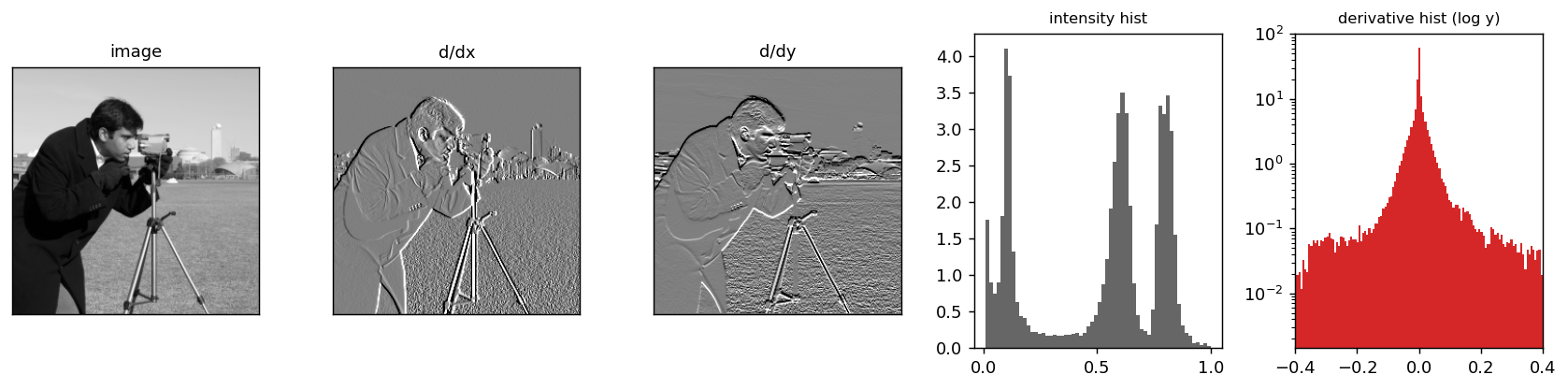
The histogram of raw intensities is broad and near-uniform, but the histogram of **image derivatives** is sharply peaked at zero with heavy tails: most of an image is smooth (derivative $\approx 0$) with rare large jumps at edges. On a log scale the derivative histogram is a **cusp**, nothing like a parabola (Gaussian).
```python theme={null}
# Figure 27.15: image, dx, dy, and the intensity vs derivative histograms.
g = to_gray_square(STREET, 256)
dx = g[:, 1:] - g[:, :-1]
dy = g[1:, :] - g[:-1, :]
```
## Derivatives are heavy-tailed, not Gaussian
The histogram of raw intensities is broad and near-uniform, but the histogram of **image derivatives** is sharply peaked at zero with heavy tails: most of an image is smooth (derivative $\approx 0$) with rare large jumps at edges. On a log scale the derivative histogram is a **cusp**, nothing like a parabola (Gaussian).
```python theme={null}
# Figure 27.15: image, dx, dy, and the intensity vs derivative histograms.
g = to_gray_square(STREET, 256)
dx = g[:, 1:] - g[:, :-1]
dy = g[1:, :] - g[:-1, :]
```
 ```python theme={null}
print('kurtosis intensity: %.1f derivative: %.1f (Gaussian = 3)'
% (_kurt(g.ravel()), _kurt(dx.ravel())))
```
```output theme={null}
kurtosis intensity: 1.7 derivative: 27.1 (Gaussian = 3)
```
## The generalized Laplacian
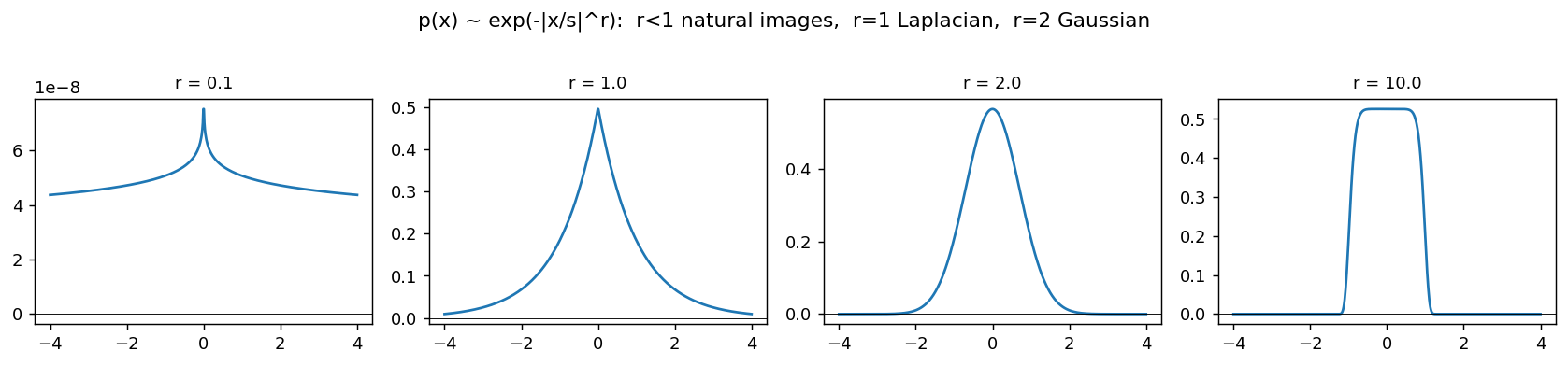
Derivative statistics are fit by the **generalized Laplacian**
$p(x)\propto \exp\!\big(-|x/s|^{\,r}\big),$
with $r\!=\!2$ Gaussian, $r\!=\!1$ Laplacian, and **$r\in[0.4,0.8]$ for natural images**: sharper peak, heavier tails than a Gaussian.
```python theme={null}
# Figure 27.17: generalized-Laplacian shapes for r = 0.1, 1, 2, 10.
x = np.linspace(-4, 4, 600)
```
```python theme={null}
print('kurtosis intensity: %.1f derivative: %.1f (Gaussian = 3)'
% (_kurt(g.ravel()), _kurt(dx.ravel())))
```
```output theme={null}
kurtosis intensity: 1.7 derivative: 27.1 (Gaussian = 3)
```
## The generalized Laplacian
Derivative statistics are fit by the **generalized Laplacian**
$p(x)\propto \exp\!\big(-|x/s|^{\,r}\big),$
with $r\!=\!2$ Gaussian, $r\!=\!1$ Laplacian, and **$r\in[0.4,0.8]$ for natural images**: sharper peak, heavier tails than a Gaussian.
```python theme={null}
# Figure 27.17: generalized-Laplacian shapes for r = 0.1, 1, 2, 10.
x = np.linspace(-4, 4, 600)
```
 ## \[1,-1] statistics: noise stays Gaussian, images do not
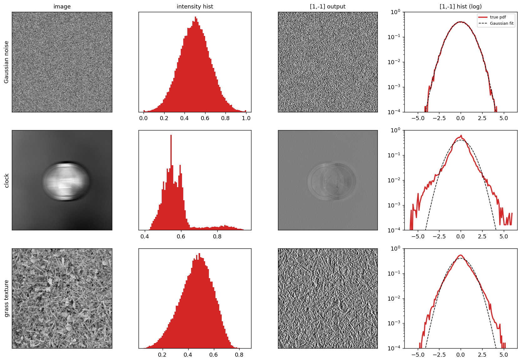
Following the book ([Figure 27.16](https://visionbook.mit.edu/stat_image_models_revised.html#fig-derivativesdistributions)), three 'visual worlds', **Gaussian noise**, a **photograph of a clock**, and a **grass texture**, are each shown with the image, its intensity histogram, its $[1,-1]$ derivative, and the derivative histogram (red) with the best Gaussian fit (black). The derivative of noise stays Gaussian; both photographs give the *same* sharply peaked, heavy-tailed shape that the Gaussian fit misses.
```python theme={null}
# Figure 27.16: image | intensity hist | [1,-1] output | output hist, x 3 worlds.
worlds = [('Gaussian noise', np.clip(0.5 + 0.15 * np.random.randn(256, 256), 0, 1)),
('clock', to_gray_square(BUILDING)),
('grass texture', to_gray_square(HAIR))]
```
## \[1,-1] statistics: noise stays Gaussian, images do not
Following the book ([Figure 27.16](https://visionbook.mit.edu/stat_image_models_revised.html#fig-derivativesdistributions)), three 'visual worlds', **Gaussian noise**, a **photograph of a clock**, and a **grass texture**, are each shown with the image, its intensity histogram, its $[1,-1]$ derivative, and the derivative histogram (red) with the best Gaussian fit (black). The derivative of noise stays Gaussian; both photographs give the *same* sharply peaked, heavy-tailed shape that the Gaussian fit misses.
```python theme={null}
# Figure 27.16: image | intensity hist | [1,-1] output | output hist, x 3 worlds.
worlds = [('Gaussian noise', np.clip(0.5 + 0.15 * np.random.randn(256, 256), 0, 1)),
('clock', to_gray_square(BUILDING)),
('grass texture', to_gray_square(HAIR))]
```
 ## Denoising with the Gaussian (1/f) prior: the Wiener filter
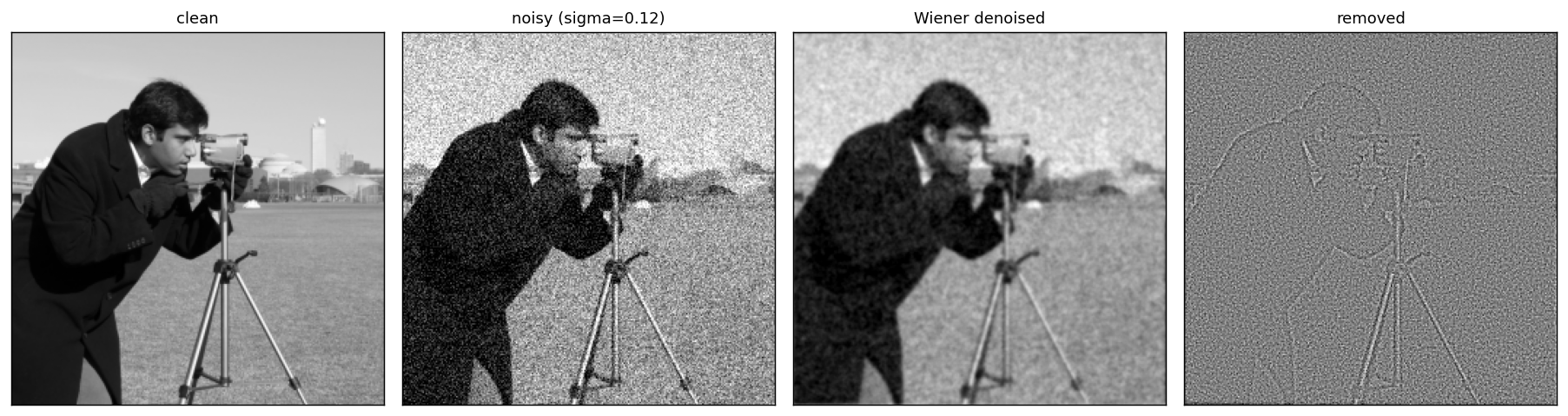
Under a Gaussian prior with power spectrum $S(w)=A/w^{2\alpha}$ and white noise of variance $\sigma^2$, the MAP estimate is the **Wiener filter**
$\mathscr L(w)=\frac{S(w)}{S(w)+\sigma^2}\,\mathscr L_g(w),$
which keeps low frequencies (where the image dominates) and suppresses high frequencies (where noise dominates). The book's version is [Figure 27.14](https://visionbook.mit.edu/stat_image_models_revised.html#fig-denoisingGaussianModel).
```python theme={null}
# Figure 27.14: clean, noisy, Wiener-denoised, and the removed noise.
g = to_gray_square(BCN, 256); sigma = 0.12
noisy = g + sigma * np.random.randn(*g.shape)
fy = np.fft.fftfreq(256)[:, None]; fx = np.fft.fftfreq(256)[None, :]
w = np.sqrt(fx**2 + fy**2) * 256 + 1e-3 # fftfreq order (unshifted)
# Wiener gain S/(S+sigma^2) for a 1/f^{2a} prior S = A/w^{2a}; writing A via the
# crossover w0 where signal power = noise power gives H = 1/(1 + (w/w0)^{2a}).
alpha, w0 = 1.5, 45.0
H = 1.0 / (1.0 + (w / w0)**(2 * alpha))
den = np.real(np.fft.ifft2(np.fft.fft2(noisy - noisy.mean()) * H)) + noisy.mean()
show = [(g, 'clean'), (noisy, 'noisy (sigma=0.12)'), (den, 'Wiener denoised'), (0.5 + (noisy - den), 'removed')]
```
## Denoising with the Gaussian (1/f) prior: the Wiener filter
Under a Gaussian prior with power spectrum $S(w)=A/w^{2\alpha}$ and white noise of variance $\sigma^2$, the MAP estimate is the **Wiener filter**
$\mathscr L(w)=\frac{S(w)}{S(w)+\sigma^2}\,\mathscr L_g(w),$
which keeps low frequencies (where the image dominates) and suppresses high frequencies (where noise dominates). The book's version is [Figure 27.14](https://visionbook.mit.edu/stat_image_models_revised.html#fig-denoisingGaussianModel).
```python theme={null}
# Figure 27.14: clean, noisy, Wiener-denoised, and the removed noise.
g = to_gray_square(BCN, 256); sigma = 0.12
noisy = g + sigma * np.random.randn(*g.shape)
fy = np.fft.fftfreq(256)[:, None]; fx = np.fft.fftfreq(256)[None, :]
w = np.sqrt(fx**2 + fy**2) * 256 + 1e-3 # fftfreq order (unshifted)
# Wiener gain S/(S+sigma^2) for a 1/f^{2a} prior S = A/w^{2a}; writing A via the
# crossover w0 where signal power = noise power gives H = 1/(1 + (w/w0)^{2a}).
alpha, w0 = 1.5, 45.0
H = 1.0 / (1.0 + (w / w0)**(2 * alpha))
den = np.real(np.fft.ifft2(np.fft.fft2(noisy - noisy.mean()) * H)) + noisy.mean()
show = [(g, 'clean'), (noisy, 'noisy (sigma=0.12)'), (den, 'Wiener denoised'), (0.5 + (noisy - den), 'removed')]
```
 ```python theme={null}
print('RMSE noisy: %.4f denoised: %.4f' % (np.sqrt(((noisy - g)**2).mean()), np.sqrt(((den - g)**2).mean())))
```
```output theme={null}
RMSE noisy: 0.1201 denoised: 0.0500
```
## Wavelet denoising as coring
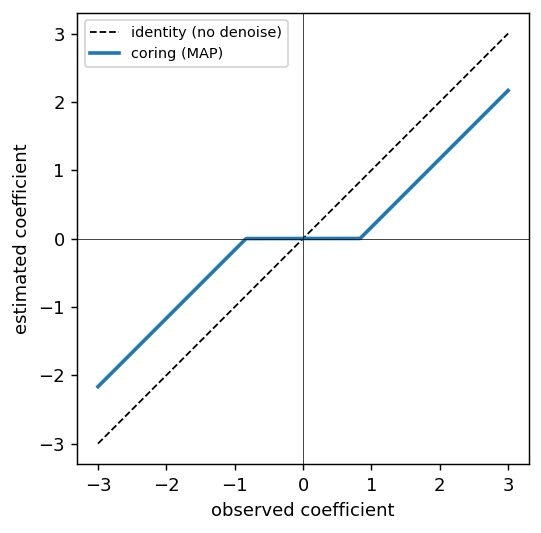
With a **Laplacian prior** on a band-pass coefficient and Gaussian noise, the MAP estimate shrinks small coefficients toward zero and leaves large ones almost untouched: a **coring** curve. Small (probably-noise) responses are cored out; strong (probably-signal) responses survive.
```python theme={null}
# Figure 27.21: the coring (shrinkage) curve for a Laplacian prior.
def coring(xhat, s=0.3, sigma=0.5):
# MAP of p(x) ~ exp(-|x|/s) * exp(-(x-xhat)^2/2sigma^2): soft-threshold by sigma^2/s.
t = sigma**2 / s
return np.sign(xhat) * np.maximum(np.abs(xhat) - t, 0.0)
xhat = np.linspace(-3, 3, 400)
```
```python theme={null}
print('RMSE noisy: %.4f denoised: %.4f' % (np.sqrt(((noisy - g)**2).mean()), np.sqrt(((den - g)**2).mean())))
```
```output theme={null}
RMSE noisy: 0.1201 denoised: 0.0500
```
## Wavelet denoising as coring
With a **Laplacian prior** on a band-pass coefficient and Gaussian noise, the MAP estimate shrinks small coefficients toward zero and leaves large ones almost untouched: a **coring** curve. Small (probably-noise) responses are cored out; strong (probably-signal) responses survive.
```python theme={null}
# Figure 27.21: the coring (shrinkage) curve for a Laplacian prior.
def coring(xhat, s=0.3, sigma=0.5):
# MAP of p(x) ~ exp(-|x|/s) * exp(-(x-xhat)^2/2sigma^2): soft-threshold by sigma^2/s.
t = sigma**2 / s
return np.sign(xhat) * np.maximum(np.abs(xhat) - t, 0.0)
xhat = np.linspace(-3, 3, 400)
```
 ## Non-local means
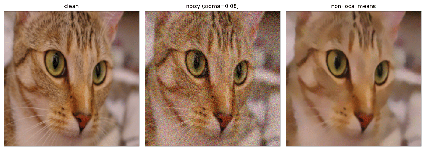
Rather than a parametric prior, **non-local means** denoises each pixel by averaging other pixels whose surrounding *patch* looks similar: a nonparametric image model. It exploits the self-similarity (repeated structure) of natural images. The book's version is [Figure 27.23](https://visionbook.mit.edu/stat_image_models_revised.html#fig-nlm2).
```python theme={null}
# Figure 27.23: clean, noisy, and non-local-means denoised (a color photo,
# shown full-frame, not center-cropped).
from skimage.restoration import denoise_nl_means
g = resize(BURANO, (232, 232), anti_aliasing=True) # full color scene
sigma = 0.08
noisy = np.clip(g + sigma * np.random.randn(*g.shape), 0, 1)
nlm = denoise_nl_means(noisy, h=0.8 * sigma, sigma=sigma, patch_size=5,
patch_distance=6, fast_mode=True, channel_axis=-1)
```
## Non-local means
Rather than a parametric prior, **non-local means** denoises each pixel by averaging other pixels whose surrounding *patch* looks similar: a nonparametric image model. It exploits the self-similarity (repeated structure) of natural images. The book's version is [Figure 27.23](https://visionbook.mit.edu/stat_image_models_revised.html#fig-nlm2).
```python theme={null}
# Figure 27.23: clean, noisy, and non-local-means denoised (a color photo,
# shown full-frame, not center-cropped).
from skimage.restoration import denoise_nl_means
g = resize(BURANO, (232, 232), anti_aliasing=True) # full color scene
sigma = 0.08
noisy = np.clip(g + sigma * np.random.randn(*g.shape), 0, 1)
nlm = denoise_nl_means(noisy, h=0.8 * sigma, sigma=sigma, patch_size=5,
patch_distance=6, fast_mode=True, channel_axis=-1)
```
 ```python theme={null}
print('RMSE noisy: %.4f NLM: %.4f' % (np.sqrt(((noisy - g)**2).mean()), np.sqrt(((nlm - g)**2).mean())))
```
```output theme={null}
RMSE noisy: 0.0794 NLM: 0.0309
```
## More representations from the chapter
The figures above cover the chapter's core arc. Below are several more of the book's representations that are worth reproducing: the *space of visual worlds* (27.2), the **dead-leaves** generative model (27.9), the role of **Fourier phase** (27.12), a **Gaussian texture** model (27.13), and how the prior shapes **reconstruction** (27.19) and **wavelet coefficient** estimation (27.20).
### Eight visual worlds
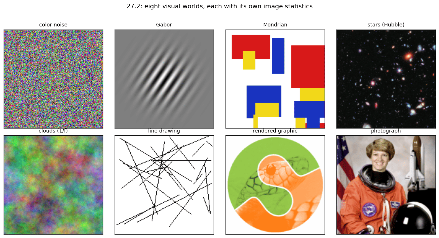
Different sources of images (noise, an oriented Gabor, a Mondrian, a star field, clouds, lines, rendered graphics, a photograph) occupy very different regions of image space, each with its own statistics. A single model cannot fit them all. The book's version is [Figure 27.2](https://visionbook.mit.edu/stat_image_models_revised.html#fig-worlds); here the eight are generated or taken from test images.
```python theme={null}
from skimage.draw import line
g = np.random.default_rng(0); S = 160
yy, xx = np.mgrid[0:S, 0:S] / S
# stand-in for the eight visual worlds in the book; original: https://visionbook.mit.edu/stat_image_models_revised.html#fig-worlds
noise = g.random((S, S, 3))
gab = 0.5 + 0.5 * np.cos(2 * np.pi * 12 * (xx * np.cos(0.6) + yy * np.sin(0.6))) * np.exp(-((xx - .5)**2 + (yy - .5)**2) / 0.05)
mondrian = np.ones((S, S, 3))
palette = np.array([[.85, .1, .1], [.1, .2, .75], [.95, .85, .1], [1, 1, 1], [.05, .05, .05]])
for _ in range(16):
y0, x0 = g.integers(0, S, 2); h, w = g.integers(15, 70, 2)
mondrian[y0:y0 + h, x0:x0 + w] = palette[g.integers(len(palette))]
drawing = np.ones((S, S, 3))
for _ in range(25):
r0, c0, r1, c1 = g.integers(0, S, 4); rr, cc = line(r0, c0, r1, c1); drawing[rr, cc] = 0
logo = img_as_float(data.logo()); cgi = logo[..., :3] * logo[..., 3:] + (1 - logo[..., 3:]) # rendered graphic on white
worlds = [(noise, 'color noise'), (np.repeat(gab[..., None], 3, -1), 'Gabor'),
(mondrian, 'Mondrian'), (resize(STARS, (S, S, 3)), 'stars (Hubble)'),
(resize(CLOUDS, (S, S, 3)), 'clouds (1/f)'), (drawing, 'line drawing'),
(resize(cgi, (S, S, 3)), 'rendered graphic'), (resize(DOME, (S, S, 3)), 'photograph')]
```
```python theme={null}
print('RMSE noisy: %.4f NLM: %.4f' % (np.sqrt(((noisy - g)**2).mean()), np.sqrt(((nlm - g)**2).mean())))
```
```output theme={null}
RMSE noisy: 0.0794 NLM: 0.0309
```
## More representations from the chapter
The figures above cover the chapter's core arc. Below are several more of the book's representations that are worth reproducing: the *space of visual worlds* (27.2), the **dead-leaves** generative model (27.9), the role of **Fourier phase** (27.12), a **Gaussian texture** model (27.13), and how the prior shapes **reconstruction** (27.19) and **wavelet coefficient** estimation (27.20).
### Eight visual worlds
Different sources of images (noise, an oriented Gabor, a Mondrian, a star field, clouds, lines, rendered graphics, a photograph) occupy very different regions of image space, each with its own statistics. A single model cannot fit them all. The book's version is [Figure 27.2](https://visionbook.mit.edu/stat_image_models_revised.html#fig-worlds); here the eight are generated or taken from test images.
```python theme={null}
from skimage.draw import line
g = np.random.default_rng(0); S = 160
yy, xx = np.mgrid[0:S, 0:S] / S
# stand-in for the eight visual worlds in the book; original: https://visionbook.mit.edu/stat_image_models_revised.html#fig-worlds
noise = g.random((S, S, 3))
gab = 0.5 + 0.5 * np.cos(2 * np.pi * 12 * (xx * np.cos(0.6) + yy * np.sin(0.6))) * np.exp(-((xx - .5)**2 + (yy - .5)**2) / 0.05)
mondrian = np.ones((S, S, 3))
palette = np.array([[.85, .1, .1], [.1, .2, .75], [.95, .85, .1], [1, 1, 1], [.05, .05, .05]])
for _ in range(16):
y0, x0 = g.integers(0, S, 2); h, w = g.integers(15, 70, 2)
mondrian[y0:y0 + h, x0:x0 + w] = palette[g.integers(len(palette))]
drawing = np.ones((S, S, 3))
for _ in range(25):
r0, c0, r1, c1 = g.integers(0, S, 4); rr, cc = line(r0, c0, r1, c1); drawing[rr, cc] = 0
logo = img_as_float(data.logo()); cgi = logo[..., :3] * logo[..., 3:] + (1 - logo[..., 3:]) # rendered graphic on white
worlds = [(noise, 'color noise'), (np.repeat(gab[..., None], 3, -1), 'Gabor'),
(mondrian, 'Mondrian'), (resize(STARS, (S, S, 3)), 'stars (Hubble)'),
(resize(CLOUDS, (S, S, 3)), 'clouds (1/f)'), (drawing, 'line drawing'),
(resize(cgi, (S, S, 3)), 'rendered graphic'), (resize(DOME, (S, S, 3)), 'photograph')]
```
 ### The dead-leaves model
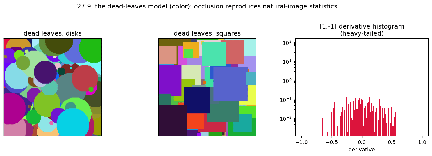
A simple *generative* model of natural images: repeatedly drop opaque colored shapes (disks and squares) of random size, each occluding what is beneath. Like the book ([Figure 27.9](https://visionbook.mit.edu/stat_image_models_revised.html#fig-deadleaves)), the figure shows a disk version and a square version. Occlusion alone reproduces hallmarks of natural-image statistics: scale-invariant structure and a **heavy-tailed** derivative histogram.
```python theme={null}
def dead_leaves(size=220, n=1600, rmin=3, rmax=40, seed=0, squares=False):
g = np.random.default_rng(seed); img = np.full((size, size, 3), 0.5)
yy, xx = np.mgrid[0:size, 0:size]
for _ in range(n):
cx, cy = g.integers(0, size, 2); r = g.integers(rmin, rmax); col = g.random(3)
m = (np.abs(xx-cx) < r) & (np.abs(yy-cy) < r) if squares else ((xx-cx)**2 + (yy-cy)**2 < r*r)
img[m] = col
return img
dl_c = dead_leaves(seed=1); dl_s = dead_leaves(seed=2, squares=True)
```
### The dead-leaves model
A simple *generative* model of natural images: repeatedly drop opaque colored shapes (disks and squares) of random size, each occluding what is beneath. Like the book ([Figure 27.9](https://visionbook.mit.edu/stat_image_models_revised.html#fig-deadleaves)), the figure shows a disk version and a square version. Occlusion alone reproduces hallmarks of natural-image statistics: scale-invariant structure and a **heavy-tailed** derivative histogram.
```python theme={null}
def dead_leaves(size=220, n=1600, rmin=3, rmax=40, seed=0, squares=False):
g = np.random.default_rng(seed); img = np.full((size, size, 3), 0.5)
yy, xx = np.mgrid[0:size, 0:size]
for _ in range(n):
cx, cy = g.integers(0, size, 2); r = g.integers(rmin, rmax); col = g.random(3)
m = (np.abs(xx-cx) < r) & (np.abs(yy-cy) < r) if squares else ((xx-cx)**2 + (yy-cy)**2 < r*r)
img[m] = col
return img
dl_c = dead_leaves(seed=1); dl_s = dead_leaves(seed=2, squares=True)
```
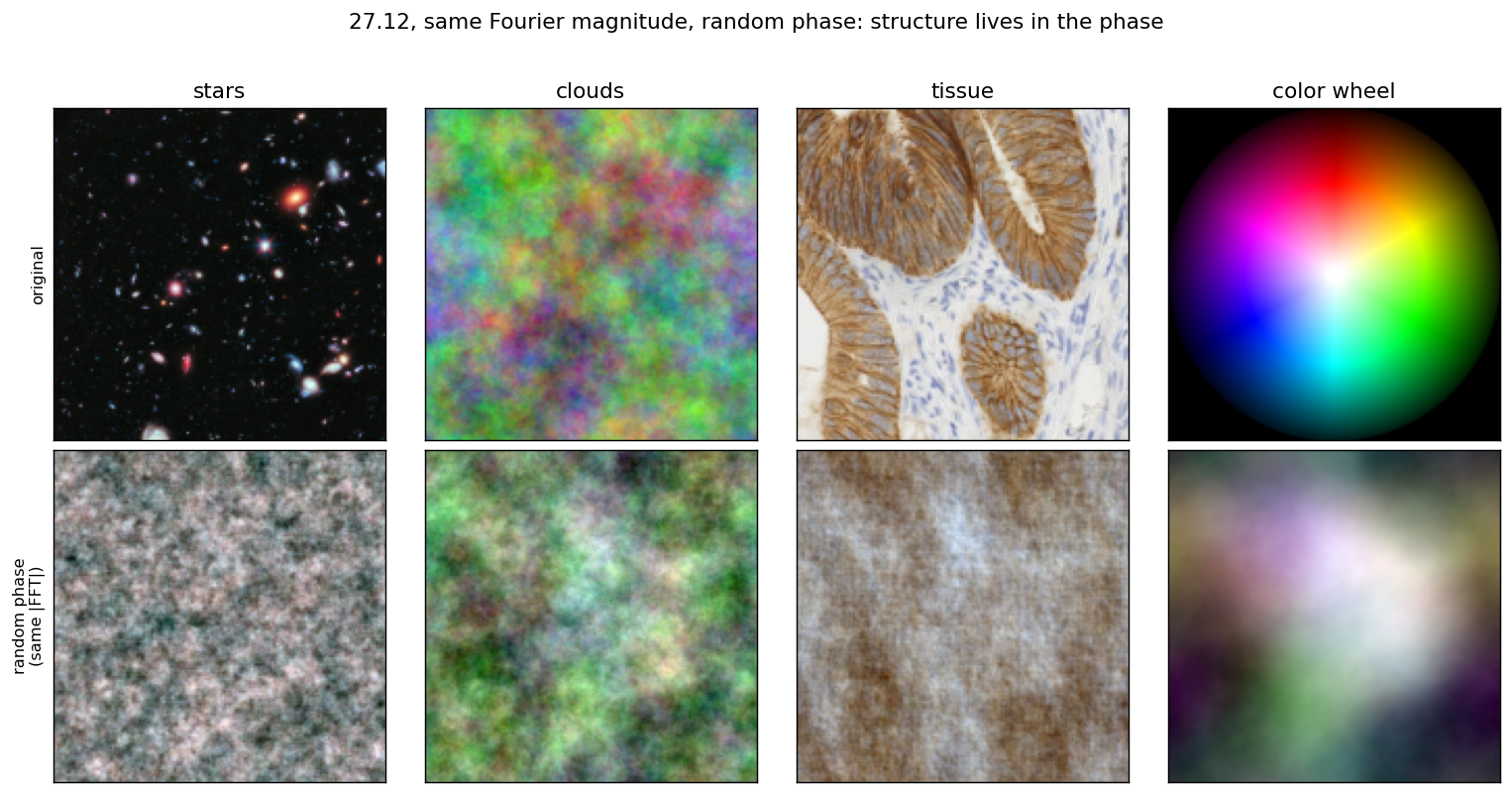
 ### Matched Fourier magnitude: phase carries the structure
The 1/f power spectrum (27.10) fixes the Fourier **magnitude**. But the magnitude alone does not make an image look like anything: keep each image's magnitude and replace its **phase** with random phase, and the recognizable content dissolves into 1/f texture. It is the **phase** that encodes edges and objects. The book's version is [Figure 27.12](https://visionbook.mit.edu/stat_image_models_revised.html#fig-magFTMatch).
```python theme={null}
def random_phase(img):
ph = np.angle(np.fft.fft2(np.random.default_rng(0).standard_normal(img.shape[:2]))) # one phase field, shared across color
out = np.zeros_like(img)
for c in range(img.shape[2]):
mag = np.abs(np.fft.fft2(img[..., c]))
out[..., c] = np.fft.ifft2(mag * np.exp(1j*ph)).real
return np.clip((out - out.min()) / (np.ptp(out) + 1e-9), 0, 1)
pairs = [('stars', STARS), ('clouds', CLOUDS), ('tissue', PLUMS), ('color wheel', CUBE)]
```
### Matched Fourier magnitude: phase carries the structure
The 1/f power spectrum (27.10) fixes the Fourier **magnitude**. But the magnitude alone does not make an image look like anything: keep each image's magnitude and replace its **phase** with random phase, and the recognizable content dissolves into 1/f texture. It is the **phase** that encodes edges and objects. The book's version is [Figure 27.12](https://visionbook.mit.edu/stat_image_models_revised.html#fig-magFTMatch).
```python theme={null}
def random_phase(img):
ph = np.angle(np.fft.fft2(np.random.default_rng(0).standard_normal(img.shape[:2]))) # one phase field, shared across color
out = np.zeros_like(img)
for c in range(img.shape[2]):
mag = np.abs(np.fft.fft2(img[..., c]))
out[..., c] = np.fft.ifft2(mag * np.exp(1j*ph)).real
return np.clip((out - out.min()) / (np.ptp(out) + 1e-9), 0, 1)
pairs = [('stars', STARS), ('clouds', CLOUDS), ('tissue', PLUMS), ('color wheel', CUBE)]
```
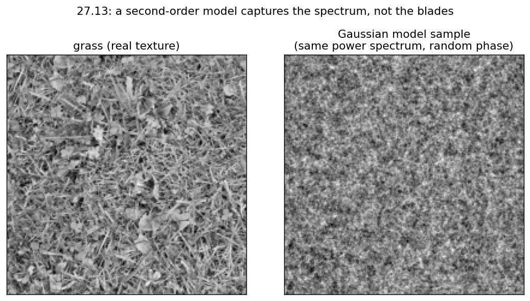
 ### A Gaussian texture model
The fully second-order (Gaussian) model of a texture keeps only the mean and the **power spectrum**, and draws a sample with random phase. The book shows this on [hair](https://visionbook.mit.edu/stat_image_models_revised.html#fig-hair); here it runs on grass, another oriented texture. The model captures the dominant orientation and scale, but having thrown away the phase, it cannot reproduce the individual **blades**; the sample looks like a phase-scrambled version.
```python theme={null}
hair = to_gray_square(HAIR, 200)
F = np.fft.fft2(hair - hair.mean()); mag = np.abs(F)
ph = np.angle(np.fft.fft2(np.random.default_rng(3).standard_normal(hair.shape)))
sample = hair.mean() + np.fft.ifft2(mag * np.exp(1j*ph)).real
```
### A Gaussian texture model
The fully second-order (Gaussian) model of a texture keeps only the mean and the **power spectrum**, and draws a sample with random phase. The book shows this on [hair](https://visionbook.mit.edu/stat_image_models_revised.html#fig-hair); here it runs on grass, another oriented texture. The model captures the dominant orientation and scale, but having thrown away the phase, it cannot reproduce the individual **blades**; the sample looks like a phase-scrambled version.
```python theme={null}
hair = to_gray_square(HAIR, 200)
F = np.fft.fft2(hair - hair.mean()); mag = np.abs(F)
ph = np.angle(np.fft.fft2(np.random.default_rng(3).standard_normal(hair.shape)))
sample = hair.mean() + np.fft.ifft2(mag * np.exp(1j*ph)).real
```
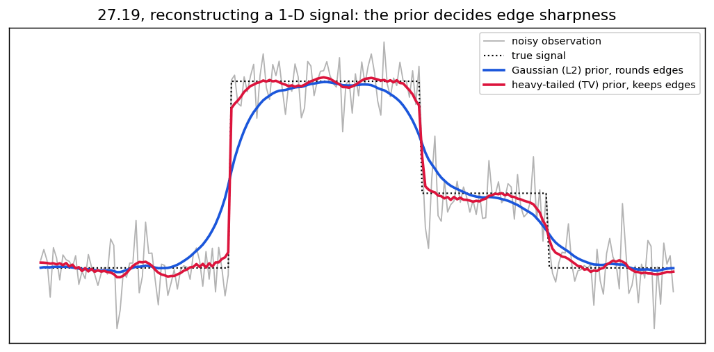
 ### The prior decides how a reconstruction looks
Reconstructing a 1-D signal from noisy samples: a **Gaussian (L2)** smoothness prior penalizes all differences quadratically and rounds off the edges; a **heavy-tailed (total-variation)** prior tolerates a few large jumps, so it keeps edges sharp while flattening the noise: the 1-D analogue of edge-preserving image denoising.
```python theme={null}
from numpy.fft import rfft, irfft
from skimage.restoration import denoise_tv_chambolle
g = np.random.default_rng(1); n = 200
sig = np.zeros(n); sig[60:120] = 1.0; sig[120:160] = 0.4
obs = sig + 0.12 * g.standard_normal(n)
w = 2*np.pi*np.fft.rfftfreq(n); l2 = irfft(rfft(obs)/(1 + 40.0*w**2), n) # Gaussian (L2) prior
tv = denoise_tv_chambolle(obs, weight=0.4) # heavy-tailed (TV) prior
```
### The prior decides how a reconstruction looks
Reconstructing a 1-D signal from noisy samples: a **Gaussian (L2)** smoothness prior penalizes all differences quadratically and rounds off the edges; a **heavy-tailed (total-variation)** prior tolerates a few large jumps, so it keeps edges sharp while flattening the noise: the 1-D analogue of edge-preserving image denoising.
```python theme={null}
from numpy.fft import rfft, irfft
from skimage.restoration import denoise_tv_chambolle
g = np.random.default_rng(1); n = 200
sig = np.zeros(n); sig[60:120] = 1.0; sig[120:160] = 0.4
obs = sig + 0.12 * g.standard_normal(n)
w = 2*np.pi*np.fft.rfftfreq(n); l2 = irfft(rfft(obs)/(1 + 40.0*w**2), n) # Gaussian (L2) prior
tv = denoise_tv_chambolle(obs, weight=0.4) # heavy-tailed (TV) prior
```
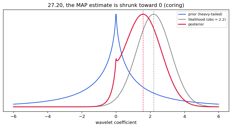
 ### Prior × likelihood = posterior for a wavelet coefficient
Estimating a single band-pass (wavelet) coefficient from a noisy measurement: the **heavy-tailed prior** (peaked at 0) multiplied by the **Gaussian likelihood** (centered on the noisy observation) gives a **posterior** whose peak is pulled back toward zero. Small coefficients are shrunk to (near) zero and large ones are kept: exactly the **coring** nonlinearity of 27.21.
```python theme={null}
x = np.linspace(-6, 6, 600); y_obs = 2.2; sigma = 1.0
prior = gen_laplacian(x, r=0.6, s=0.7); prior /= prior.max()
like = np.exp(-(x - y_obs)**2 / (2*sigma**2)); like /= like.max()
post = prior * like; post /= post.max()
```
### Prior × likelihood = posterior for a wavelet coefficient
Estimating a single band-pass (wavelet) coefficient from a noisy measurement: the **heavy-tailed prior** (peaked at 0) multiplied by the **Gaussian likelihood** (centered on the noisy observation) gives a **posterior** whose peak is pulled back toward zero. Small coefficients are shrunk to (near) zero and large ones are kept: exactly the **coring** nonlinearity of 27.21.
```python theme={null}
x = np.linspace(-6, 6, 600); y_obs = 2.2; sigma = 1.0
prior = gen_laplacian(x, r=0.6, s=0.7); prior /= prior.max()
like = np.exp(-(x - y_obs)**2 / (2*sigma**2)); like /= like.max()
post = prior * like; post /= post.max()
```
 ## Concluding remarks
| Statistic / model | What it captures | Use |
| - | - | - |
| $1/w^{\alpha}$ power law | second-order (Fourier) structure | Gaussian prior, Wiener denoising |
| pixel-correlation decay | short-range dependence | why iid pixels fail |
| generalized Laplacian of derivatives | heavy tails / sparsity | wavelet coring |
| non-local self-similarity | repeated structure | non-local means |
Natural images occupy a tiny, structured sliver of image space. Measuring that structure, a power law here, heavy-tailed derivatives there, gives priors that turn ill-posed problems (denoising, inpainting, super-resolution) into tractable Bayesian estimates, and sets the stage for the learned generative models later in the book.
***
[Edit this page on GitHub](https://github.com/aegean-ai/eaia/edit/main/src/aiml-common/lectures/image-processing/statistical-image-models/index.mdx) or [file an issue](https://github.com/aegean-ai/eaia/issues/new/choose).
## Concluding remarks
| Statistic / model | What it captures | Use |
| - | - | - |
| $1/w^{\alpha}$ power law | second-order (Fourier) structure | Gaussian prior, Wiener denoising |
| pixel-correlation decay | short-range dependence | why iid pixels fail |
| generalized Laplacian of derivatives | heavy tails / sparsity | wavelet coring |
| non-local self-similarity | repeated structure | non-local means |
Natural images occupy a tiny, structured sliver of image space. Measuring that structure, a power law here, heavy-tailed derivatives there, gives priors that turn ill-posed problems (denoising, inpainting, super-resolution) into tractable Bayesian estimates, and sets the stage for the learned generative models later in the book.
***
[Edit this page on GitHub](https://github.com/aegean-ai/eaia/edit/main/src/aiml-common/lectures/image-processing/statistical-image-models/index.mdx) or [file an issue](https://github.com/aegean-ai/eaia/issues/new/choose).