> ## Documentation Index
> Fetch the complete documentation index at: https://aegean.ai/llms.txt
> Use this file to discover all available pages before exploring further.
# Filtering in Space and Time
> A video as a space-time volume: motion as orientation, spatiotemporal Gaussians, velocity-tuned blur, and velocity-nulling filters.
 *This section was written by [Kaushik Kachireddy](https://github.com/kaushik0x7d2) ([pull request #78](https://github.com/pantelis/eng-ai-agents/pull/78)), with help from an AI coding agent (Claude Code) on the code. It reproduces the ideas of Chapter 19 of [*Foundations of Computer Vision*](https://visionbook.mit.edu/temporal_filters_v2.html) by Antonio Torralba, Phillip Isola, and William T. Freeman.*
A video is a 3D volume $\ell(x,y,t)$. Once you think of it that way, **motion becomes orientation**: a static point is a vertical line in the $x$-$t$ slice, and a point moving at velocity $v$ is a line of slope $1/v$.
This section builds the chapter's space-time tools on a **real pedestrian video**, a static-camera clip of people crossing a plaza (OpenCV's `vtest.avi` sample), the same kind of scene the book uses ([Figure 19.1](https://visionbook.mit.edu/temporal_filters_v2.html#fig-motion)). It covers the $x$-$t$ view of motion, its space-time Fourier signature, the **spatiotemporal Gaussian** and its velocity-skewed form, **velocity-tuned blur**, spatiotemporal derivatives, and the **velocity-nulling filter** that erases objects moving at a chosen velocity.
```python theme={null}
import numpy as np
import torch
import torch.nn.functional as F
import matplotlib.pyplot as plt
np.random.seed(0); _ = torch.manual_seed(0)
```
```python theme={null}
# ---- real pedestrian sequence: OpenCV's vtest.avi (static camera, people walking) ----
# 56 color frames pre-extracted and downsampled to a compact file, so no video decoder
# is needed at run time. Static camera -> background is fixed, people move.
import os, urllib.request
SEQ_URL = ('https://raw.githubusercontent.com/pantelis/eng-ai-agents/main/notebooks/CV/'
'mit-foundations/chapter-19-temporal-filters/assets/ped_seq.npz')
_cands = ['assets/ped_seq.npz',
'notebooks/CV/mit-foundations/chapter-19-temporal-filters/assets/ped_seq.npz']
_path = next((p for p in _cands if os.path.exists(p)), None)
if _path is None: # not next to this section: download it once
_path = 'ped_seq.npz'
if not os.path.exists(_path):
urllib.request.urlretrieve(SEQ_URL, _path)
SEQ = np.load(_path)['seq'].astype(np.float32) / 255.0
P, H, W = SEQ.shape[:3] # (frames, height, width)
MROW = int(0.55 * H) # x-t slice row, through the walking people
print('sequence:', SEQ.shape, ' frames:', P)
```
```output theme={null}
sequence: (56, 120, 160, 3) frames: 56
```
## A video is a space-time volume
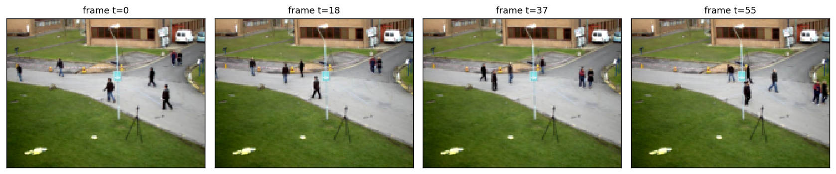
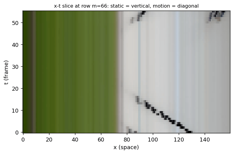
Stacking the frames along $t$ gives a 3-D volume. Slice it at a fixed row $m$ and you get an **$x$-$t$ image**: the static background is made of vertical streaks (same $x$ for every $t$), while each walking person traces a **diagonal streak** whose slope is its velocity. This is the whole idea of the chapter: motion has become orientation.
```python theme={null}
# Figure 19.1: frames (top) and the x-t slice (motion = diagonal streaks).
idx = [0, P // 3, 2 * P // 3, P - 1]
show([SEQ[i] for i in idx], [f'frame t={i}' for i in idx], figsize=(13, 3.0))
xt = SEQ[:, MROW, :, :] # (P, W, 3): rows = t, cols = x
```
*This section was written by [Kaushik Kachireddy](https://github.com/kaushik0x7d2) ([pull request #78](https://github.com/pantelis/eng-ai-agents/pull/78)), with help from an AI coding agent (Claude Code) on the code. It reproduces the ideas of Chapter 19 of [*Foundations of Computer Vision*](https://visionbook.mit.edu/temporal_filters_v2.html) by Antonio Torralba, Phillip Isola, and William T. Freeman.*
A video is a 3D volume $\ell(x,y,t)$. Once you think of it that way, **motion becomes orientation**: a static point is a vertical line in the $x$-$t$ slice, and a point moving at velocity $v$ is a line of slope $1/v$.
This section builds the chapter's space-time tools on a **real pedestrian video**, a static-camera clip of people crossing a plaza (OpenCV's `vtest.avi` sample), the same kind of scene the book uses ([Figure 19.1](https://visionbook.mit.edu/temporal_filters_v2.html#fig-motion)). It covers the $x$-$t$ view of motion, its space-time Fourier signature, the **spatiotemporal Gaussian** and its velocity-skewed form, **velocity-tuned blur**, spatiotemporal derivatives, and the **velocity-nulling filter** that erases objects moving at a chosen velocity.
```python theme={null}
import numpy as np
import torch
import torch.nn.functional as F
import matplotlib.pyplot as plt
np.random.seed(0); _ = torch.manual_seed(0)
```
```python theme={null}
# ---- real pedestrian sequence: OpenCV's vtest.avi (static camera, people walking) ----
# 56 color frames pre-extracted and downsampled to a compact file, so no video decoder
# is needed at run time. Static camera -> background is fixed, people move.
import os, urllib.request
SEQ_URL = ('https://raw.githubusercontent.com/pantelis/eng-ai-agents/main/notebooks/CV/'
'mit-foundations/chapter-19-temporal-filters/assets/ped_seq.npz')
_cands = ['assets/ped_seq.npz',
'notebooks/CV/mit-foundations/chapter-19-temporal-filters/assets/ped_seq.npz']
_path = next((p for p in _cands if os.path.exists(p)), None)
if _path is None: # not next to this section: download it once
_path = 'ped_seq.npz'
if not os.path.exists(_path):
urllib.request.urlretrieve(SEQ_URL, _path)
SEQ = np.load(_path)['seq'].astype(np.float32) / 255.0
P, H, W = SEQ.shape[:3] # (frames, height, width)
MROW = int(0.55 * H) # x-t slice row, through the walking people
print('sequence:', SEQ.shape, ' frames:', P)
```
```output theme={null}
sequence: (56, 120, 160, 3) frames: 56
```
## A video is a space-time volume
Stacking the frames along $t$ gives a 3-D volume. Slice it at a fixed row $m$ and you get an **$x$-$t$ image**: the static background is made of vertical streaks (same $x$ for every $t$), while each walking person traces a **diagonal streak** whose slope is its velocity. This is the whole idea of the chapter: motion has become orientation.
```python theme={null}
# Figure 19.1: frames (top) and the x-t slice (motion = diagonal streaks).
idx = [0, P // 3, 2 * P // 3, P - 1]
show([SEQ[i] for i in idx], [f'frame t={i}' for i in idx], figsize=(13, 3.0))
xt = SEQ[:, MROW, :, :] # (P, W, 3): rows = t, cols = x
```
 ## Motion is a slanted plane in the Fourier domain
A globally translating image $\ell(x,y,t)=\ell_0(x-v_xt,\,y-v_yt)$ has all its energy on the plane
$w_t + v_x w_x + v_y w_y = 0.$
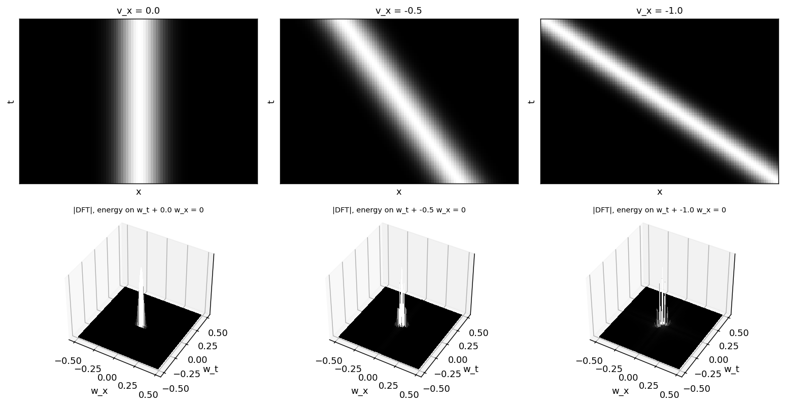
In 1-D space, a pulse moving at velocity $v$ is a slanted band in $x$-$t$, and its 2-D Fourier transform is a **sinc ridge lying along the line $w_t+v\,w_x=0$**: vertical for a static pulse, tilting as the speed grows.
```python theme={null}
# Figure 19.2: moving 1D pulse (top) and its space-time |DFT| (bottom).
Wp, Pp = 96, 96
def moving_pulse(v, width=6):
xt = np.zeros((Pp, Wp))
xs = np.arange(Wp)
for t in range(Pp):
c = Wp * 0.5 + v * (t - Pp / 2)
xt[t] = np.exp(-((xs - c) ** 2) / (2 * width ** 2))
return xt
vs = [0.0, -0.5, -1.0]
```
## Motion is a slanted plane in the Fourier domain
A globally translating image $\ell(x,y,t)=\ell_0(x-v_xt,\,y-v_yt)$ has all its energy on the plane
$w_t + v_x w_x + v_y w_y = 0.$
In 1-D space, a pulse moving at velocity $v$ is a slanted band in $x$-$t$, and its 2-D Fourier transform is a **sinc ridge lying along the line $w_t+v\,w_x=0$**: vertical for a static pulse, tilting as the speed grows.
```python theme={null}
# Figure 19.2: moving 1D pulse (top) and its space-time |DFT| (bottom).
Wp, Pp = 96, 96
def moving_pulse(v, width=6):
xt = np.zeros((Pp, Wp))
xs = np.arange(Wp)
for t in range(Pp):
c = Wp * 0.5 + v * (t - Pp / 2)
xt[t] = np.exp(-((xs - c) ** 2) / (2 * width ** 2))
return xt
vs = [0.0, -0.5, -1.0]
```
 ## The spatiotemporal Gaussian
The separable space-time Gaussian
$g(x,y,t;\sigma,\sigma_t)=\tfrac{1}{(2\pi)^{3/2}\sigma^2\sigma_t} e^{-(x^2+y^2)/2\sigma^2}\,e^{-t^2/2\sigma_t^2}$
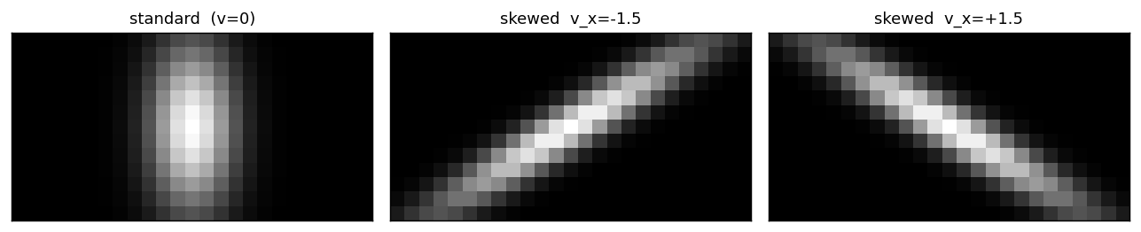
is an isotropic blob in $x$-$t$. **Skewing** it along a velocity, $g(x-v_xt,\,y-v_yt,\,t)$, tilts the blob so its long axis follows that motion. Convolving with the skewed kernel is what blurs *along* a velocity.
```python theme={null}
# Kernel builders on a 3D (t, y, x) grid.
def st_grid(rt, ry, rx):
t = np.arange(-rt, rt + 1); y = np.arange(-ry, ry + 1); x = np.arange(-rx, rx + 1)
return np.meshgrid(t, y, x, indexing='ij') # T, Y, X
def st_gaussian(sig, sigt, rt, ry, rx, vx=0.0, vy=0.0):
T, Y, X = st_grid(rt, ry, rx)
xs, ys = X - vx * T, Y - vy * T # shear by velocity
g = np.exp(-(xs**2 + ys**2) / (2 * sig**2)) * np.exp(-T**2 / (2 * sigt**2))
return g / g.sum()
def st_deriv(sig, sigt, axis, rt, ry, rx):
T, Y, X = st_grid(rt, ry, rx)
g = np.exp(-(X**2 + Y**2) / (2 * sig**2)) * np.exp(-T**2 / (2 * sigt**2))
g = g / g.sum()
return {'t': -T / sigt**2, 'x': -X / sig**2, 'y': -Y / sig**2}[axis] * g
# Figure 19.3: x-t central slice (y=0) of the Gaussian: standard vs velocity-skewed.
rt, ry, rx = 6, 4, 12 # wide in x so the skew fits
kernels = [('standard (v=0)', st_gaussian(2.0, 4.0, rt, ry, rx)),
('skewed v_x=-1.5', st_gaussian(2.0, 4.0, rt, ry, rx, vx=-1.5)),
('skewed v_x=+1.5', st_gaussian(2.0, 4.0, rt, ry, rx, vx=1.5))]
show([k[:, ry, :] for _, k in kernels], [n for n, _ in kernels], figsize=(10, 3.4))
print('each kernel sums to 1:', [round(float(k.sum()), 3) for _, k in kernels])
```
## The spatiotemporal Gaussian
The separable space-time Gaussian
$g(x,y,t;\sigma,\sigma_t)=\tfrac{1}{(2\pi)^{3/2}\sigma^2\sigma_t} e^{-(x^2+y^2)/2\sigma^2}\,e^{-t^2/2\sigma_t^2}$
is an isotropic blob in $x$-$t$. **Skewing** it along a velocity, $g(x-v_xt,\,y-v_yt,\,t)$, tilts the blob so its long axis follows that motion. Convolving with the skewed kernel is what blurs *along* a velocity.
```python theme={null}
# Kernel builders on a 3D (t, y, x) grid.
def st_grid(rt, ry, rx):
t = np.arange(-rt, rt + 1); y = np.arange(-ry, ry + 1); x = np.arange(-rx, rx + 1)
return np.meshgrid(t, y, x, indexing='ij') # T, Y, X
def st_gaussian(sig, sigt, rt, ry, rx, vx=0.0, vy=0.0):
T, Y, X = st_grid(rt, ry, rx)
xs, ys = X - vx * T, Y - vy * T # shear by velocity
g = np.exp(-(xs**2 + ys**2) / (2 * sig**2)) * np.exp(-T**2 / (2 * sigt**2))
return g / g.sum()
def st_deriv(sig, sigt, axis, rt, ry, rx):
T, Y, X = st_grid(rt, ry, rx)
g = np.exp(-(X**2 + Y**2) / (2 * sig**2)) * np.exp(-T**2 / (2 * sigt**2))
g = g / g.sum()
return {'t': -T / sigt**2, 'x': -X / sig**2, 'y': -Y / sig**2}[axis] * g
# Figure 19.3: x-t central slice (y=0) of the Gaussian: standard vs velocity-skewed.
rt, ry, rx = 6, 4, 12 # wide in x so the skew fits
kernels = [('standard (v=0)', st_gaussian(2.0, 4.0, rt, ry, rx)),
('skewed v_x=-1.5', st_gaussian(2.0, 4.0, rt, ry, rx, vx=-1.5)),
('skewed v_x=+1.5', st_gaussian(2.0, 4.0, rt, ry, rx, vx=1.5))]
show([k[:, ry, :] for _, k in kernels], [n for n, _ in kernels], figsize=(10, 3.4))
print('each kernel sums to 1:', [round(float(k.sum()), 3) for _, k in kernels])
```
 ```output theme={null}
each kernel sums to 1: [1.0, 1.0, 1.0]
```
## Velocity-tuned (temporal) blur
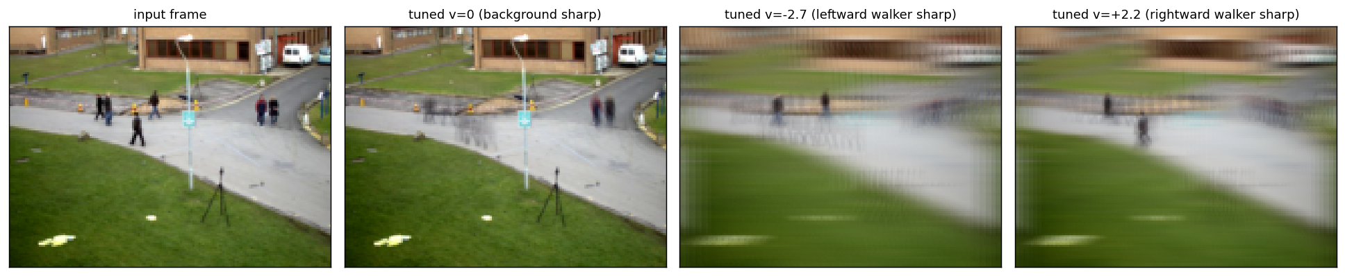
Averaging the volume **along a velocity** keeps whatever moves at that velocity sharp (it sits still in the motion-compensated stack) while everything else smears. Tuning to $v=0$ keeps the **static background** crisp and blurs the walkers; tuning to a walker's velocity makes **that walker** snap into focus while the background streaks.
```python theme={null}
def conv3d_seq(vol, kernel):
"""Convolve a single-channel (P,H,W) volume with a (kt,kh,kw) kernel."""
x = torch.from_numpy(vol).float()[None, None]
k = torch.from_numpy(kernel).float()[None, None]
kt, kh, kw = kernel.shape
x = F.pad(x, (kw // 2, kw // 2, kh // 2, kh // 2, kt // 2, kt // 2), mode='replicate')
return F.conv3d(x, k)[0, 0].numpy()
def conv3d_rgb(seq, kernel):
return np.stack([conv3d_seq(seq[..., c], kernel) for c in range(3)], axis=-1)
def velocity_blur(seq, vx, vy, rt=6, sigt=4.0):
"""Motion-compensated temporal blur: Gaussian-average the frames after shifting
each by the velocity, so an object moving at (vx,vy) stays aligned (sharp) while
the rest smears. Fast shift-and-add, avoids a huge sheared 3D kernel.
"""
dts = np.arange(-rt, rt + 1)
w = np.exp(-dts**2 / (2 * sigt**2)); w = w / w.sum()
Pn = seq.shape[0]; out = np.zeros_like(seq)
for dt, wt in zip(dts, w):
fr = seq[np.clip(np.arange(Pn) + dt, 0, Pn - 1)]
fr = np.roll(fr, (int(round(vy * dt)), int(round(vx * dt))), axis=(1, 2))
out += wt * fr
return out
# Figure 19.4: temporal blur tuned to different velocities (which stays sharp?).
blur0 = velocity_blur(SEQ, 0.0, 0.0) # tuned to static background
blurL = velocity_blur(SEQ, -2.7, 0.0) # tuned to a leftward walker
blurR = velocity_blur(SEQ, 2.2, 0.0) # tuned to a rightward walker
fr = P // 2
show([SEQ[fr], blur0[fr], blurL[fr], blurR[fr]],
['input frame', 'tuned v=0 (background sharp)', 'tuned v=-2.7 (leftward walker sharp)', 'tuned v=+2.2 (rightward walker sharp)'],
figsize=(15, 3.0))
```
```output theme={null}
each kernel sums to 1: [1.0, 1.0, 1.0]
```
## Velocity-tuned (temporal) blur
Averaging the volume **along a velocity** keeps whatever moves at that velocity sharp (it sits still in the motion-compensated stack) while everything else smears. Tuning to $v=0$ keeps the **static background** crisp and blurs the walkers; tuning to a walker's velocity makes **that walker** snap into focus while the background streaks.
```python theme={null}
def conv3d_seq(vol, kernel):
"""Convolve a single-channel (P,H,W) volume with a (kt,kh,kw) kernel."""
x = torch.from_numpy(vol).float()[None, None]
k = torch.from_numpy(kernel).float()[None, None]
kt, kh, kw = kernel.shape
x = F.pad(x, (kw // 2, kw // 2, kh // 2, kh // 2, kt // 2, kt // 2), mode='replicate')
return F.conv3d(x, k)[0, 0].numpy()
def conv3d_rgb(seq, kernel):
return np.stack([conv3d_seq(seq[..., c], kernel) for c in range(3)], axis=-1)
def velocity_blur(seq, vx, vy, rt=6, sigt=4.0):
"""Motion-compensated temporal blur: Gaussian-average the frames after shifting
each by the velocity, so an object moving at (vx,vy) stays aligned (sharp) while
the rest smears. Fast shift-and-add, avoids a huge sheared 3D kernel.
"""
dts = np.arange(-rt, rt + 1)
w = np.exp(-dts**2 / (2 * sigt**2)); w = w / w.sum()
Pn = seq.shape[0]; out = np.zeros_like(seq)
for dt, wt in zip(dts, w):
fr = seq[np.clip(np.arange(Pn) + dt, 0, Pn - 1)]
fr = np.roll(fr, (int(round(vy * dt)), int(round(vx * dt))), axis=(1, 2))
out += wt * fr
return out
# Figure 19.4: temporal blur tuned to different velocities (which stays sharp?).
blur0 = velocity_blur(SEQ, 0.0, 0.0) # tuned to static background
blurL = velocity_blur(SEQ, -2.7, 0.0) # tuned to a leftward walker
blurR = velocity_blur(SEQ, 2.2, 0.0) # tuned to a rightward walker
fr = P // 2
show([SEQ[fr], blur0[fr], blurL[fr], blurR[fr]],
['input frame', 'tuned v=0 (background sharp)', 'tuned v=-2.7 (leftward walker sharp)', 'tuned v=+2.2 (rightward walker sharp)'],
figsize=(15, 3.0))
```
 ## Spatiotemporal Gaussian derivatives
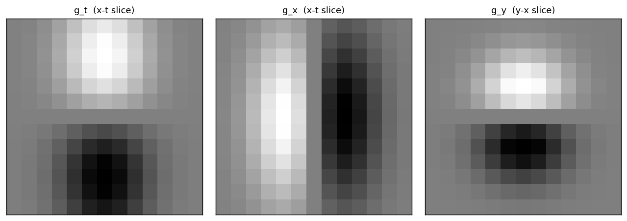
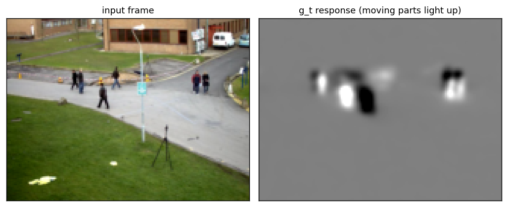
The space-time gradient $\nabla g=(g_x,g_y,g_t)$ gives oriented derivative filters. The **temporal** derivative $g_t=-\tfrac{t}{\sigma_t^2}g$ responds to change over time: it is large exactly where something moves and zero on the static background.
```python theme={null}
# Figure 19.5/19.6: g_t and the spatial derivatives as slices, and g_t on a frame.
gt = st_deriv(2.0, 4.0, 't', 6, 6, 6)
gx = st_deriv(2.0, 4.0, 'x', 6, 6, 6)
gy = st_deriv(2.0, 4.0, 'y', 6, 6, 6)
show([show_signed(gt[:, 6, :]), show_signed(gx[:, 6, :]), show_signed(gy[6, :, :])],
['g_t (x-t slice)', 'g_x (x-t slice)', 'g_y (y-x slice)'], figsize=(10, 3.4))
gray = SEQ.mean(-1) # luminance volume
gt_small = st_deriv(2.0, 4.0, 't', 6, 4, 4) # smaller spatial support -> faster
resp_t = conv3d_seq(gray, gt_small) # temporal-derivative response
fr = P // 2
show([SEQ[fr], show_signed(resp_t[fr])],
['input frame', 'g_t response (moving parts light up)'], figsize=(8, 3.2))
```
## Spatiotemporal Gaussian derivatives
The space-time gradient $\nabla g=(g_x,g_y,g_t)$ gives oriented derivative filters. The **temporal** derivative $g_t=-\tfrac{t}{\sigma_t^2}g$ responds to change over time: it is large exactly where something moves and zero on the static background.
```python theme={null}
# Figure 19.5/19.6: g_t and the spatial derivatives as slices, and g_t on a frame.
gt = st_deriv(2.0, 4.0, 't', 6, 6, 6)
gx = st_deriv(2.0, 4.0, 'x', 6, 6, 6)
gy = st_deriv(2.0, 4.0, 'y', 6, 6, 6)
show([show_signed(gt[:, 6, :]), show_signed(gx[:, 6, :]), show_signed(gy[6, :, :])],
['g_t (x-t slice)', 'g_x (x-t slice)', 'g_y (y-x slice)'], figsize=(10, 3.4))
gray = SEQ.mean(-1) # luminance volume
gt_small = st_deriv(2.0, 4.0, 't', 6, 4, 4) # smaller spatial support -> faster
resp_t = conv3d_seq(gray, gt_small) # temporal-derivative response
fr = P // 2
show([SEQ[fr], show_signed(resp_t[fr])],
['input frame', 'g_t response (moving parts light up)'], figsize=(8, 3.2))
```
 ## The velocity-nulling filter
By the brightness-constancy relation, an image moving at exactly $(v_x,v_y)$ satisfies $\partial_t\ell + v_x\partial_x\ell + v_y\partial_y\ell = 0$. So the filter
$h = g_t + v_x g_x + v_y g_y$
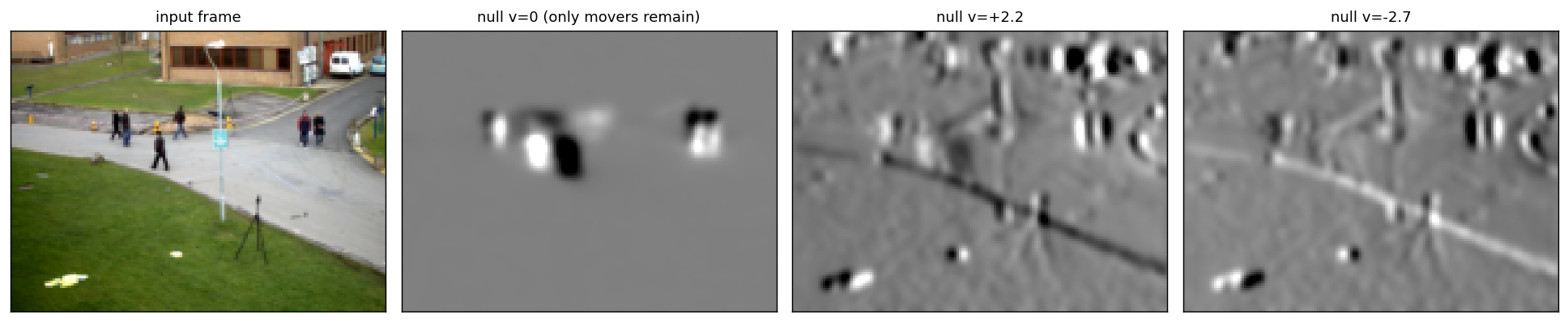
**annihilates** anything moving at $(v_x,v_y)$ while passing everything else. Nulling $v=0$ removes the **static background** (only the walkers survive); nulling a walker's velocity erases *that* walker while the rest remain.
```python theme={null}
# Figure 19.7: velocity-nulling on the x-t slice and on a frame.
def null_kernel(vx, vy):
return (st_deriv(2.0, 4.0, 't', 6, 4, 4)
+ vx * st_deriv(2.0, 4.0, 'x', 6, 4, 4)
+ vy * st_deriv(2.0, 4.0, 'y', 6, 4, 4))
gray = SEQ.mean(-1)
outs = {v: conv3d_seq(gray, null_kernel(v, 0.0)) for v in (0.0, 2.2, -2.7)}
# x-t slices (top): the streak matching the null velocity disappears.
show([show_signed(gray[:, MROW, :]),
show_signed(outs[0.0][:, MROW, :]),
show_signed(outs[2.2][:, MROW, :]),
show_signed(outs[-2.7][:, MROW, :])],
['x-t input', 'null v=0 (static gone)', 'null v=+2.2', 'null v=-2.7'],
figsize=(15, 3.2))
fr = P // 2
show([SEQ[fr], show_signed(outs[0.0][fr]), show_signed(outs[2.2][fr]), show_signed(outs[-2.7][fr])],
['input frame', 'null v=0 (only movers remain)', 'null v=+2.2', 'null v=-2.7'], figsize=(15, 3.0))
# Nulling v=0 = pure g_t: static background is driven near zero.
print('static-background energy: input %.4f -> after null v=0 %.4f'
% (float(np.abs(gray - gray.mean()).mean()), float(np.abs(outs[0.0]).mean())))
```
## The velocity-nulling filter
By the brightness-constancy relation, an image moving at exactly $(v_x,v_y)$ satisfies $\partial_t\ell + v_x\partial_x\ell + v_y\partial_y\ell = 0$. So the filter
$h = g_t + v_x g_x + v_y g_y$
**annihilates** anything moving at $(v_x,v_y)$ while passing everything else. Nulling $v=0$ removes the **static background** (only the walkers survive); nulling a walker's velocity erases *that* walker while the rest remain.
```python theme={null}
# Figure 19.7: velocity-nulling on the x-t slice and on a frame.
def null_kernel(vx, vy):
return (st_deriv(2.0, 4.0, 't', 6, 4, 4)
+ vx * st_deriv(2.0, 4.0, 'x', 6, 4, 4)
+ vy * st_deriv(2.0, 4.0, 'y', 6, 4, 4))
gray = SEQ.mean(-1)
outs = {v: conv3d_seq(gray, null_kernel(v, 0.0)) for v in (0.0, 2.2, -2.7)}
# x-t slices (top): the streak matching the null velocity disappears.
show([show_signed(gray[:, MROW, :]),
show_signed(outs[0.0][:, MROW, :]),
show_signed(outs[2.2][:, MROW, :]),
show_signed(outs[-2.7][:, MROW, :])],
['x-t input', 'null v=0 (static gone)', 'null v=+2.2', 'null v=-2.7'],
figsize=(15, 3.2))
fr = P // 2
show([SEQ[fr], show_signed(outs[0.0][fr]), show_signed(outs[2.2][fr]), show_signed(outs[-2.7][fr])],
['input frame', 'null v=0 (only movers remain)', 'null v=+2.2', 'null v=-2.7'], figsize=(15, 3.0))
# Nulling v=0 = pure g_t: static background is driven near zero.
print('static-background energy: input %.4f -> after null v=0 %.4f'
% (float(np.abs(gray - gray.mean()).mean()), float(np.abs(outs[0.0]).mean())))
```

 ```output theme={null}
static-background energy: input 0.1824 -> after null v=0 0.0011
```
## Concluding remarks
| Tool | Space-time form | Effect |
| - | - | - |
| video volume | $\ell(x,y,t)$ | motion becomes orientation in $x$-$t$ |
| Fourier | energy on $w_t+v_xw_x+v_yw_y=0$ | speed = tilt of the spectral plane |
| spatiotemporal Gaussian | $g(x,y,t)$, skewable by $v$ | isotropic or velocity-tuned blur |
| temporal derivative | $g_t=-t/\sigma_t^2\,g$ | lights up whatever moves |
| nulling filter | $g_t+v_xg_x+v_yg_y$ | erases objects moving at $(v_x,v_y)$ |
Treating time as a third axis turns motion problems into geometry: the same Gaussian, derivative, and steering ideas from the spatial chapters carry over, and the brightness-constancy constraint becomes a single linear filter that can select or reject a velocity. These are the foundations for [motion estimation](/aiml-common/lectures/3d-reconstruction/motion-estimation/index) and optical flow.
***
[Edit this page on GitHub](https://github.com/aegean-ai/eaia/edit/main/src/aiml-common/lectures/image-processing/temporal-filters/index.mdx) or [file an issue](https://github.com/aegean-ai/eaia/issues/new/choose).
```output theme={null}
static-background energy: input 0.1824 -> after null v=0 0.0011
```
## Concluding remarks
| Tool | Space-time form | Effect |
| - | - | - |
| video volume | $\ell(x,y,t)$ | motion becomes orientation in $x$-$t$ |
| Fourier | energy on $w_t+v_xw_x+v_yw_y=0$ | speed = tilt of the spectral plane |
| spatiotemporal Gaussian | $g(x,y,t)$, skewable by $v$ | isotropic or velocity-tuned blur |
| temporal derivative | $g_t=-t/\sigma_t^2\,g$ | lights up whatever moves |
| nulling filter | $g_t+v_xg_x+v_yg_y$ | erases objects moving at $(v_x,v_y)$ |
Treating time as a third axis turns motion problems into geometry: the same Gaussian, derivative, and steering ideas from the spatial chapters carry over, and the brightness-constancy constraint becomes a single linear filter that can select or reject a velocity. These are the foundations for [motion estimation](/aiml-common/lectures/3d-reconstruction/motion-estimation/index) and optical flow.
***
[Edit this page on GitHub](https://github.com/aegean-ai/eaia/edit/main/src/aiml-common/lectures/image-processing/temporal-filters/index.mdx) or [file an issue](https://github.com/aegean-ai/eaia/issues/new/choose).