> ## Documentation Index
> Fetch the complete documentation index at: https://aegean.ai/llms.txt
> Use this file to discover all available pages before exploring further.
# Covariance, correlation, and whitening
> Covariance and correlation matrices, standardization, and PCA/ZCA whitening in PyTorch.
 ```python theme={null}
import torch
import matplotlib.pyplot as plt
torch.manual_seed(0)
def cov_matrix(X):
"""Population covariance with features in columns: Xc^T Xc / n."""
Xc = X - X.mean(dim=0, keepdim=True)
return (Xc.T @ Xc) / X.shape[0]
```
## Variance and covariance
Variance measures how a single feature spreads around its mean; covariance measures how two
features vary together. For a data matrix $X$ with $n$ rows (observations) and features in the
columns, center each column and the covariance matrix is
$\Sigma = \frac{1}{n}\, X_c^\top X_c, \qquad X_c = X - \bar{X}.$
The diagonal holds the per-feature variances; the off-diagonal entry $(i,j)$ is the covariance
between features $i$ and $j$.
```python theme={null}
A = torch.tensor([[1., 3., 5.],
[5., 4., 1.],
[3., 8., 6.]])
manual = cov_matrix(A) # features in columns
builtin = torch.cov(A.T, correction=0) # torch.cov expects variables in rows; correction=0 -> /n
print("manual:\n", manual)
print("torch.cov:\n", builtin)
assert torch.allclose(manual, builtin, atol=1e-5)
print("OK: Xc^T Xc / n equals torch.cov")
```
```output theme={null}
manual:
tensor([[ 2.6667, 0.6667, -2.6667],
[ 0.6667, 4.6667, 2.3333],
[-2.6667, 2.3333, 4.6667]])
torch.cov:
tensor([[ 2.6667, 0.6667, -2.6667],
[ 0.6667, 4.6667, 2.3333],
[-2.6667, 2.3333, 4.6667]])
OK: Xc^T Xc / n equals torch.cov
```
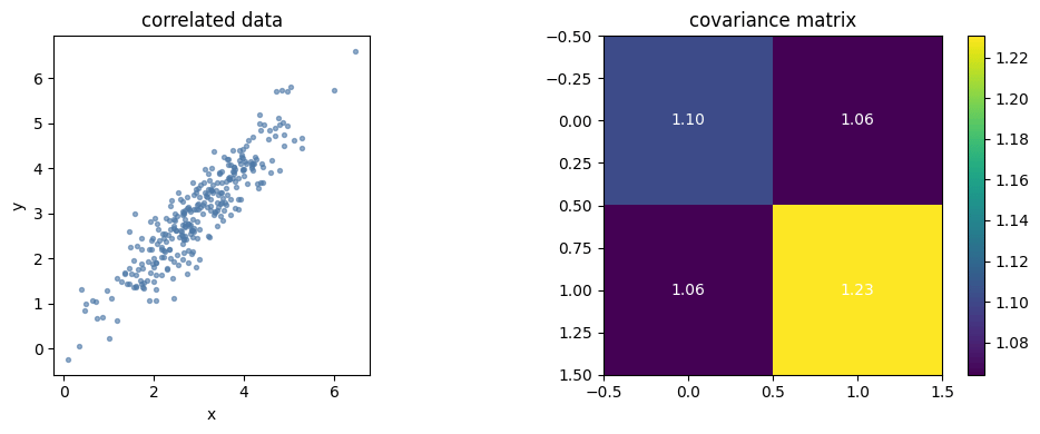
## Visualizing data and its covariance
A scatter plot shows the shape of a two-dimensional dataset, and a heatmap of its covariance
matrix shows the same structure numerically: bright off-diagonal entries mean the two features
move together.
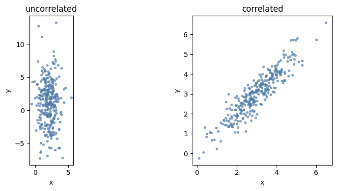
## Simulating data
Start with two independent Gaussian features: the scatter is an axis-aligned cloud and the
covariance is nearly diagonal. Then build a dependent pair, where one feature is a noisy copy of
the other: the cloud tilts and the off-diagonal covariance grows.
```python theme={null}
# Uncorrelated: two independent Gaussian features
a1 = torch.normal(2.0, 1.0, (300,))
a2 = torch.normal(1.0, 3.0, (300,))
uncorrelated = torch.stack([a1, a2], dim=1)
# Correlated: second feature is the first plus noise
b1 = torch.normal(3.0, 1.0, (300,))
b2 = b1 + torch.normal(0.0, 1.0, (300,)) * 0.5
correlated = torch.stack([b1, b2], dim=1)
print("uncorrelated off-diagonal:", cov_matrix(uncorrelated)[0, 1].item())
print("correlated off-diagonal:", cov_matrix(correlated)[0, 1].item())
assert cov_matrix(correlated)[0, 1] > cov_matrix(uncorrelated)[0, 1].abs()
```
```output theme={null}
uncorrelated off-diagonal: -0.07187948375940323
correlated off-diagonal: 1.06403648853302
```
```python theme={null}
import torch
import matplotlib.pyplot as plt
torch.manual_seed(0)
def cov_matrix(X):
"""Population covariance with features in columns: Xc^T Xc / n."""
Xc = X - X.mean(dim=0, keepdim=True)
return (Xc.T @ Xc) / X.shape[0]
```
## Variance and covariance
Variance measures how a single feature spreads around its mean; covariance measures how two
features vary together. For a data matrix $X$ with $n$ rows (observations) and features in the
columns, center each column and the covariance matrix is
$\Sigma = \frac{1}{n}\, X_c^\top X_c, \qquad X_c = X - \bar{X}.$
The diagonal holds the per-feature variances; the off-diagonal entry $(i,j)$ is the covariance
between features $i$ and $j$.
```python theme={null}
A = torch.tensor([[1., 3., 5.],
[5., 4., 1.],
[3., 8., 6.]])
manual = cov_matrix(A) # features in columns
builtin = torch.cov(A.T, correction=0) # torch.cov expects variables in rows; correction=0 -> /n
print("manual:\n", manual)
print("torch.cov:\n", builtin)
assert torch.allclose(manual, builtin, atol=1e-5)
print("OK: Xc^T Xc / n equals torch.cov")
```
```output theme={null}
manual:
tensor([[ 2.6667, 0.6667, -2.6667],
[ 0.6667, 4.6667, 2.3333],
[-2.6667, 2.3333, 4.6667]])
torch.cov:
tensor([[ 2.6667, 0.6667, -2.6667],
[ 0.6667, 4.6667, 2.3333],
[-2.6667, 2.3333, 4.6667]])
OK: Xc^T Xc / n equals torch.cov
```
## Visualizing data and its covariance
A scatter plot shows the shape of a two-dimensional dataset, and a heatmap of its covariance
matrix shows the same structure numerically: bright off-diagonal entries mean the two features
move together.
## Simulating data
Start with two independent Gaussian features: the scatter is an axis-aligned cloud and the
covariance is nearly diagonal. Then build a dependent pair, where one feature is a noisy copy of
the other: the cloud tilts and the off-diagonal covariance grows.
```python theme={null}
# Uncorrelated: two independent Gaussian features
a1 = torch.normal(2.0, 1.0, (300,))
a2 = torch.normal(1.0, 3.0, (300,))
uncorrelated = torch.stack([a1, a2], dim=1)
# Correlated: second feature is the first plus noise
b1 = torch.normal(3.0, 1.0, (300,))
b2 = b1 + torch.normal(0.0, 1.0, (300,)) * 0.5
correlated = torch.stack([b1, b2], dim=1)
print("uncorrelated off-diagonal:", cov_matrix(uncorrelated)[0, 1].item())
print("correlated off-diagonal:", cov_matrix(correlated)[0, 1].item())
assert cov_matrix(correlated)[0, 1] > cov_matrix(uncorrelated)[0, 1].abs()
```
```output theme={null}
uncorrelated off-diagonal: -0.07187948375940323
correlated off-diagonal: 1.06403648853302
```
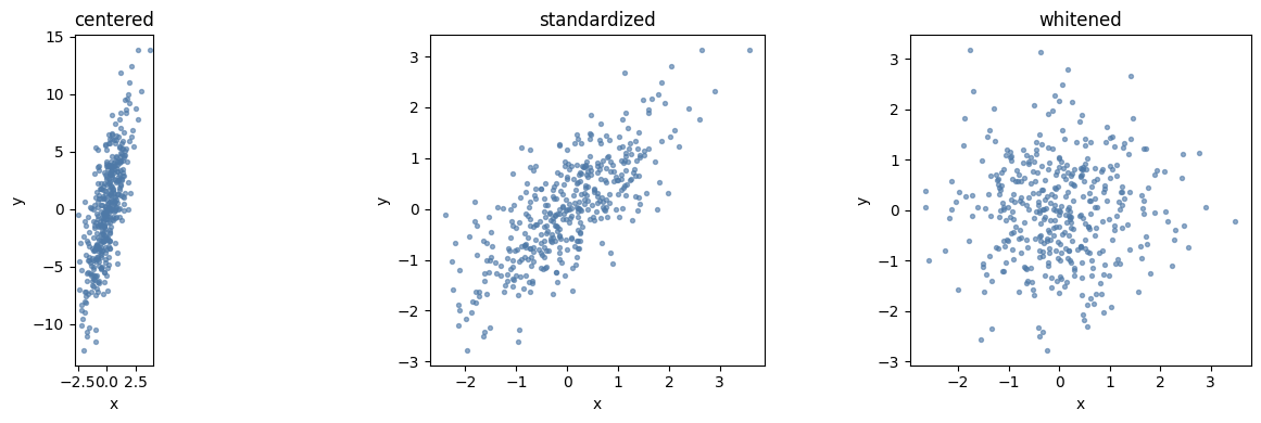
 ## Preprocessing: centering, standardization, and whitening
Centering subtracts the per-feature mean. Standardization additionally divides by the
per-feature standard deviation, putting every feature on the same scale. Whitening goes further:
it removes the correlations between features so that the covariance matrix becomes the identity.
Whitening has three steps: center the data, rotate it onto the eigenvectors of the covariance
matrix (which decorrelates it), then rescale each new axis by $1/\sqrt{\lambda + \epsilon}$, where
$\lambda$ is the corresponding eigenvalue and $\epsilon$ is a small stabilizer.
```python theme={null}
def center(X):
return X - X.mean(dim=0, keepdim=True)
def standardize(X):
return center(X) / X.std(dim=0, unbiased=False, keepdim=True)
def whiten(X, eps=1e-5):
Xc = center(X)
cov = (Xc.T @ Xc) / Xc.shape[0]
eigvals, eigvecs = torch.linalg.eigh(cov) # cov is symmetric PSD
Xrot = Xc @ eigvecs # decorrelate (rotate onto eigenbasis)
return Xrot / torch.sqrt(eigvals + eps) # rescale each axis to unit variance
# Build a correlated dataset with different per-feature scales
c1 = torch.normal(3.0, 1.0, (400,))
c2 = (c1 + torch.normal(0.0, 1.0, (400,))) * 3.0
C = torch.stack([c1, c2], dim=1)
Cw = whiten(C)
cov_white = cov_matrix(Cw)
print("covariance after whitening:\n", cov_white)
assert torch.allclose(cov_white, torch.eye(2), atol=1e-3)
print("OK: whitening produces (approximately) identity covariance")
```
```output theme={null}
covariance after whitening:
tensor([[ 9.9998e-01, -1.2308e-07],
[-1.2308e-07, 1.0000e+00]])
OK: whitening produces (approximately) identity covariance
```
## Preprocessing: centering, standardization, and whitening
Centering subtracts the per-feature mean. Standardization additionally divides by the
per-feature standard deviation, putting every feature on the same scale. Whitening goes further:
it removes the correlations between features so that the covariance matrix becomes the identity.
Whitening has three steps: center the data, rotate it onto the eigenvectors of the covariance
matrix (which decorrelates it), then rescale each new axis by $1/\sqrt{\lambda + \epsilon}$, where
$\lambda$ is the corresponding eigenvalue and $\epsilon$ is a small stabilizer.
```python theme={null}
def center(X):
return X - X.mean(dim=0, keepdim=True)
def standardize(X):
return center(X) / X.std(dim=0, unbiased=False, keepdim=True)
def whiten(X, eps=1e-5):
Xc = center(X)
cov = (Xc.T @ Xc) / Xc.shape[0]
eigvals, eigvecs = torch.linalg.eigh(cov) # cov is symmetric PSD
Xrot = Xc @ eigvecs # decorrelate (rotate onto eigenbasis)
return Xrot / torch.sqrt(eigvals + eps) # rescale each axis to unit variance
# Build a correlated dataset with different per-feature scales
c1 = torch.normal(3.0, 1.0, (400,))
c2 = (c1 + torch.normal(0.0, 1.0, (400,))) * 3.0
C = torch.stack([c1, c2], dim=1)
Cw = whiten(C)
cov_white = cov_matrix(Cw)
print("covariance after whitening:\n", cov_white)
assert torch.allclose(cov_white, torch.eye(2), atol=1e-3)
print("OK: whitening produces (approximately) identity covariance")
```
```output theme={null}
covariance after whitening:
tensor([[ 9.9998e-01, -1.2308e-07],
[-1.2308e-07, 1.0000e+00]])
OK: whitening produces (approximately) identity covariance
```
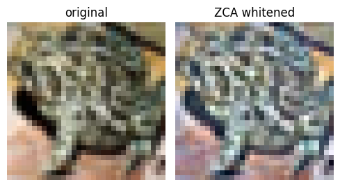
 ## Image whitening with ZCA
Whitening extends to images. Each image is a high-dimensional vector (here a 32 by 32 color
image, so 3072 values). Zero-phase component analysis (ZCA) whitening decorrelates the pixel
dimensions while keeping the result as close as possible to the original image, so the whitened
picture still looks like the scene with its local structure emphasized. The ZCA transform is
$X_{\text{ZCA}} = X_c\, U\, \mathrm{diag}\!\left(\tfrac{1}{\sqrt{S + \epsilon}}\right) U^\top,$
where $U$ and $S$ come from the singular value decomposition of the pixel covariance matrix.
```python theme={null}
from datasets import load_dataset
from torchvision.transforms.functional import pil_to_tensor
ds = load_dataset("uoft-cs/cifar10", split="train[:1000]")
X = torch.stack([pil_to_tensor(im) for im in ds["img"]]).float() / 255.0 # (1000, 3, 32, 32)
X_flat = X.reshape(X.shape[0], -1) # (1000, 3072)
print("image tensor:", tuple(X.shape), "flattened:", tuple(X_flat.shape))
```
```output theme={null}
image tensor: (1000, 3, 32, 32) flattened: (1000, 3072)
```
```python theme={null}
Xc = X_flat - X_flat.mean(dim=0, keepdim=True) # per-pixel mean subtraction
cov = (Xc.T @ Xc) / Xc.shape[0] # (3072, 3072)
U, S, _ = torch.linalg.svd(cov)
eps = 0.1
zca = U @ torch.diag(1.0 / torch.sqrt(S + eps)) @ U.T
X_zca = Xc @ zca.T
print("ZCA matrix:", tuple(zca.shape))
```
```output theme={null}
ZCA matrix: (3072, 3072)
```
## Image whitening with ZCA
Whitening extends to images. Each image is a high-dimensional vector (here a 32 by 32 color
image, so 3072 values). Zero-phase component analysis (ZCA) whitening decorrelates the pixel
dimensions while keeping the result as close as possible to the original image, so the whitened
picture still looks like the scene with its local structure emphasized. The ZCA transform is
$X_{\text{ZCA}} = X_c\, U\, \mathrm{diag}\!\left(\tfrac{1}{\sqrt{S + \epsilon}}\right) U^\top,$
where $U$ and $S$ come from the singular value decomposition of the pixel covariance matrix.
```python theme={null}
from datasets import load_dataset
from torchvision.transforms.functional import pil_to_tensor
ds = load_dataset("uoft-cs/cifar10", split="train[:1000]")
X = torch.stack([pil_to_tensor(im) for im in ds["img"]]).float() / 255.0 # (1000, 3, 32, 32)
X_flat = X.reshape(X.shape[0], -1) # (1000, 3072)
print("image tensor:", tuple(X.shape), "flattened:", tuple(X_flat.shape))
```
```output theme={null}
image tensor: (1000, 3, 32, 32) flattened: (1000, 3072)
```
```python theme={null}
Xc = X_flat - X_flat.mean(dim=0, keepdim=True) # per-pixel mean subtraction
cov = (Xc.T @ Xc) / Xc.shape[0] # (3072, 3072)
U, S, _ = torch.linalg.svd(cov)
eps = 0.1
zca = U @ torch.diag(1.0 / torch.sqrt(S + eps)) @ U.T
X_zca = Xc @ zca.T
print("ZCA matrix:", tuple(zca.shape))
```
```output theme={null}
ZCA matrix: (3072, 3072)
```
 ## References
* N. Pal and S. Sudeep, "Preprocessing for image classification by convolutional neural
networks," 2016.
* A. Krizhevsky, "Learning Multiple Layers of Features from Tiny Images," 2009 (the CIFAR-10
dataset).
* See also the [whitening lecture](/aiml-common/lectures/optimization/whitening) for how
whitening relates to batch normalization, and the
[Gaussians page](/aiml-common/lectures/ml-math/probability/gaussians/gaussians) for the
distribution this section preprocesses.
***
[Edit this page on GitHub](https://github.com/aegean-ai/eaia/edit/main/src/aiml-common/lectures/ml-math/probability/gaussians/corr-cov-matrix/index.mdx) or [file an issue](https://github.com/aegean-ai/eaia/issues/new/choose).
## References
* N. Pal and S. Sudeep, "Preprocessing for image classification by convolutional neural
networks," 2016.
* A. Krizhevsky, "Learning Multiple Layers of Features from Tiny Images," 2009 (the CIFAR-10
dataset).
* See also the [whitening lecture](/aiml-common/lectures/optimization/whitening) for how
whitening relates to batch normalization, and the
[Gaussians page](/aiml-common/lectures/ml-math/probability/gaussians/gaussians) for the
distribution this section preprocesses.
***
[Edit this page on GitHub](https://github.com/aegean-ai/eaia/edit/main/src/aiml-common/lectures/ml-math/probability/gaussians/corr-cov-matrix/index.mdx) or [file an issue](https://github.com/aegean-ai/eaia/issues/new/choose).