> ## Documentation Index
> Fetch the complete documentation index at: https://aegean.ai/llms.txt
> Use this file to discover all available pages before exploring further.
# Probability Basics
> Fundamental probability concepts for machine learning.
If the contents in this section are new to you, we recommend starting with Stanford's [Probability for Computer Scientists (CS109)](https://probabilitycoders.stanford.edu/spr26).
Note also the Khan Academy [Statistics and Probability](https://www.khanacademy.org/math/statistics-probability) course, especially [Unit 7: Probability](https://www.khanacademy.org/math/statistics-probability/probability-library) and [Unit 9: Random variables](https://www.khanacademy.org/math/statistics-probability/random-variables-stats-library).
1. The whole purpose of probabilistic modeling is to introduce uncertainty into our problem statement. There are three types of uncertainties, which fall into the broader [aleatoric and epistemic](/aiml-common/lectures/aleatoric-epistemic/index) categories:
* Inherent stochasticity - e.g. impact of wind in self-driving car control systems at moderate to high speed.
* Incomplete observability - e.g. sensor imperfections causing loss of sensing information
* Incomplete modeling - e.g. models and algorithms that are not implementable to an analog world and need to be discretized.
2. Probabilities can be used in two ways.
* Probabilities can describe frequencies of outcomes in random experiments
* Probabilities can also be used, more generally, to describe degrees of belief in propositions that do not involve random variables. This more general use of probability to quantify beliefs is known as the Bayesian viewpoint. It is also known as the subjective interpretation of probability, since the probabilities depend on assumptions.
The three important probabilities that we need to be concerned with in data mining are the joint, marginal and conditional probabilities. The pictures below present some examples that we will go through.
*Discrete probability distribution function (pdf). On the right side is what is called a Hinton diagram where the area of the square represents the probability in a way that the sum equals to 1.0.*
*A more complicated discrete probability distribution over the letters of the English alphabet (letter 27 symbolizes space) as measured by reading the Linux FAQ document.*
*Continuous probability distribution density function (pdf) - the area under the curve equals 1.0*
*Joint probability $P(x,y)$ distribution over the 27x27 possible bigrams $xy$ found in the Linux FAQ document.*
*(e) and (f) represent joint distributions of discrete and continuous random variables*
## Sum and Product rules
The following video explains the sum and product rules that are extensivbely used in data science and for understanding the Bayes rule.
### Sum rule and the Marginal Probability
Given the joint what is the marginal probability $P(x)$ ?
$P(x) = \sum_y P(x,y) = \sum_y P(x | y)P(y)$
*Extracting the marginal out of the joint*
### Conditional Probability and the Product or chain rule
This is obtained from the definition of conditional probability:
$P(x,y) = P(x | y)P(y) = P(y | x)P(x)$
*Conditional probability distribution over the 27x27 possible bigrams $xy$ found in the Linux FAQ document.*
Are $x$ and $y$ in the example above independent?
**Key references**: (Kendall & Gal, 2017; Kendall & Gal, 2017; Frazier, 2018)
## References
* Frazier, P. (2018). *A Tutorial on Bayesian Optimization*.
* Kendall, A., Gal, Y. (2017). *What uncertainties do we need in Bayesian deep learning for computer vision?*.
* Kendall, A., Gal, Y. (2017). *What Uncertainties Do We Need in Bayesian Deep Learning for Computer Vision?*.
***
[Edit this page on GitHub](https://github.com/aegean-ai/eaia/edit/main/src/aiml-common/lectures/ml-math/probability/index.mdx) or [file an issue](https://github.com/aegean-ai/eaia/issues/new/choose).
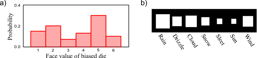 *Discrete probability distribution function (pdf). On the right side is what is called a Hinton diagram where the area of the square represents the probability in a way that the sum equals to 1.0.*
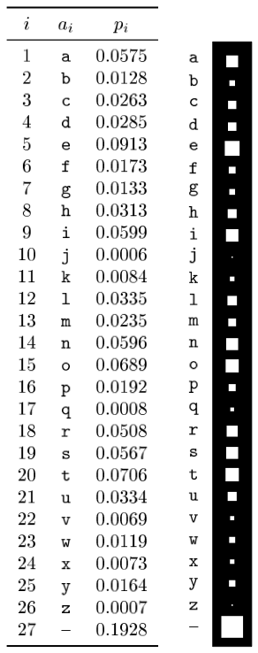 *A more complicated discrete probability distribution over the letters of the English alphabet (letter 27 symbolizes space) as measured by reading the Linux FAQ document.*
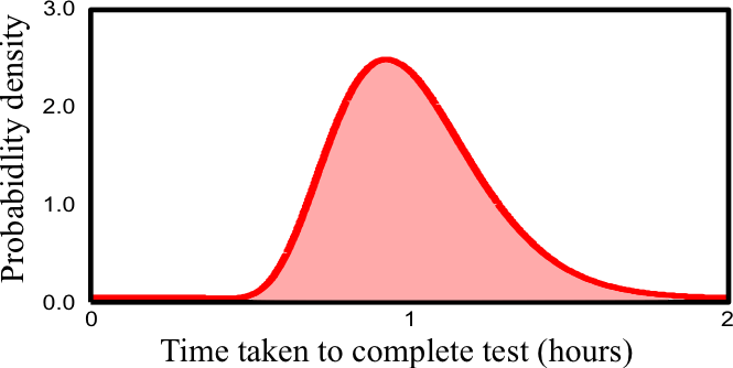 *Continuous probability distribution density function (pdf) - the area under the curve equals 1.0*
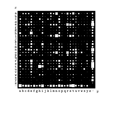 *Joint probability $P(x,y)$ distribution over the 27x27 possible bigrams $xy$ found in the Linux FAQ document.*
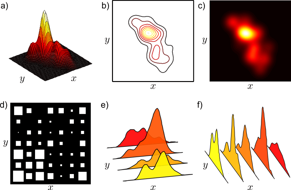 *(e) and (f) represent joint distributions of discrete and continuous random variables*
## Sum and Product rules
The following video explains the sum and product rules that are extensivbely used in data science and for understanding the Bayes rule.
### Sum rule and the Marginal Probability
Given the joint what is the marginal probability $P(x)$ ?
$P(x) = \sum_y P(x,y) = \sum_y P(x | y)P(y)$
*(e) and (f) represent joint distributions of discrete and continuous random variables*
## Sum and Product rules
The following video explains the sum and product rules that are extensivbely used in data science and for understanding the Bayes rule.
### Sum rule and the Marginal Probability
Given the joint what is the marginal probability $P(x)$ ?
$P(x) = \sum_y P(x,y) = \sum_y P(x | y)P(y)$
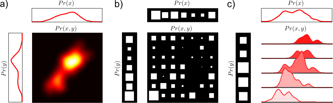 *Extracting the marginal out of the joint*
### Conditional Probability and the Product or chain rule
This is obtained from the definition of conditional probability:
$P(x,y) = P(x | y)P(y) = P(y | x)P(x)$
*Extracting the marginal out of the joint*
### Conditional Probability and the Product or chain rule
This is obtained from the definition of conditional probability:
$P(x,y) = P(x | y)P(y) = P(y | x)P(x)$
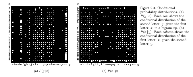 *Conditional probability distribution over the 27x27 possible bigrams $xy$ found in the Linux FAQ document.*