> ## Documentation Index
> Fetch the complete documentation index at: https://aegean.ai/llms.txt
> Use this file to discover all available pages before exploring further.
# Configuration Space Topology
> Links, joints, and configuration spaces of robots.
This section draws heavily on chapter 2, Configuration Space, of Kevin Lynch and Frank Park, *Modern Robotics: Mechanics, Planning, and Control* (Cambridge University Press, 2017). You can [download the chapter as a PDF](https://artifacts.aegeanai.com/pdf/lynch-mr/config-space.pdf).
A robot consists of bodies called links, which are connected by joints. Actuators, such as electric motors, apply forces or torques that move the links. An end-effector, such as a gripper or hand, is usually attached to one link for grasping and manipulating objects.
A robot’s *configuration* specifies the positions of all points in its mechanisms.
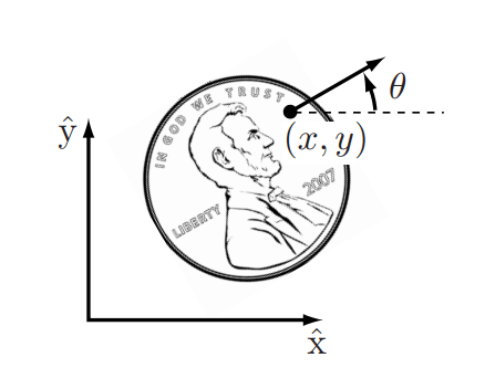
Consider a coin lying heads up on a table. Such an object is a *planar* rigid body. A *spatial* rigid body can move anywhere in three-dimensional space. Three real numbers, also called coordinates, describe the coin's configuration. Two coordinates $(x,y)$ locate a chosen point on the coin, and one coordinate ($θ$) specifies its orientation. If the coin may also lie tails up, the visible face is part of its configuration. This value belongs to the discrete set $\{\text{heads}, \text{tails}\}$ rather than a continuous range of real numbers.
You can place the coin anywhere on the table, which gives two degrees of freedom for the $(x,y)$ coordinates. The point alone does not fix the coin's configuration. If the chosen point is Abraham Lincoln's eye, for example, the coin can still rotate through 360 degrees. The angle $\theta$ describes this additional degree of freedom.
The number of degrees of freedom (dof) of a robot is the *smallest* number of real-valued coordinates needed to represent its configuration. The discrete choice of face adds no degree of freedom. The coin has $f=3$ degrees of freedom. Its current configuration is one point in the space of all its possible configurations, called the *configuration space* (C-space).
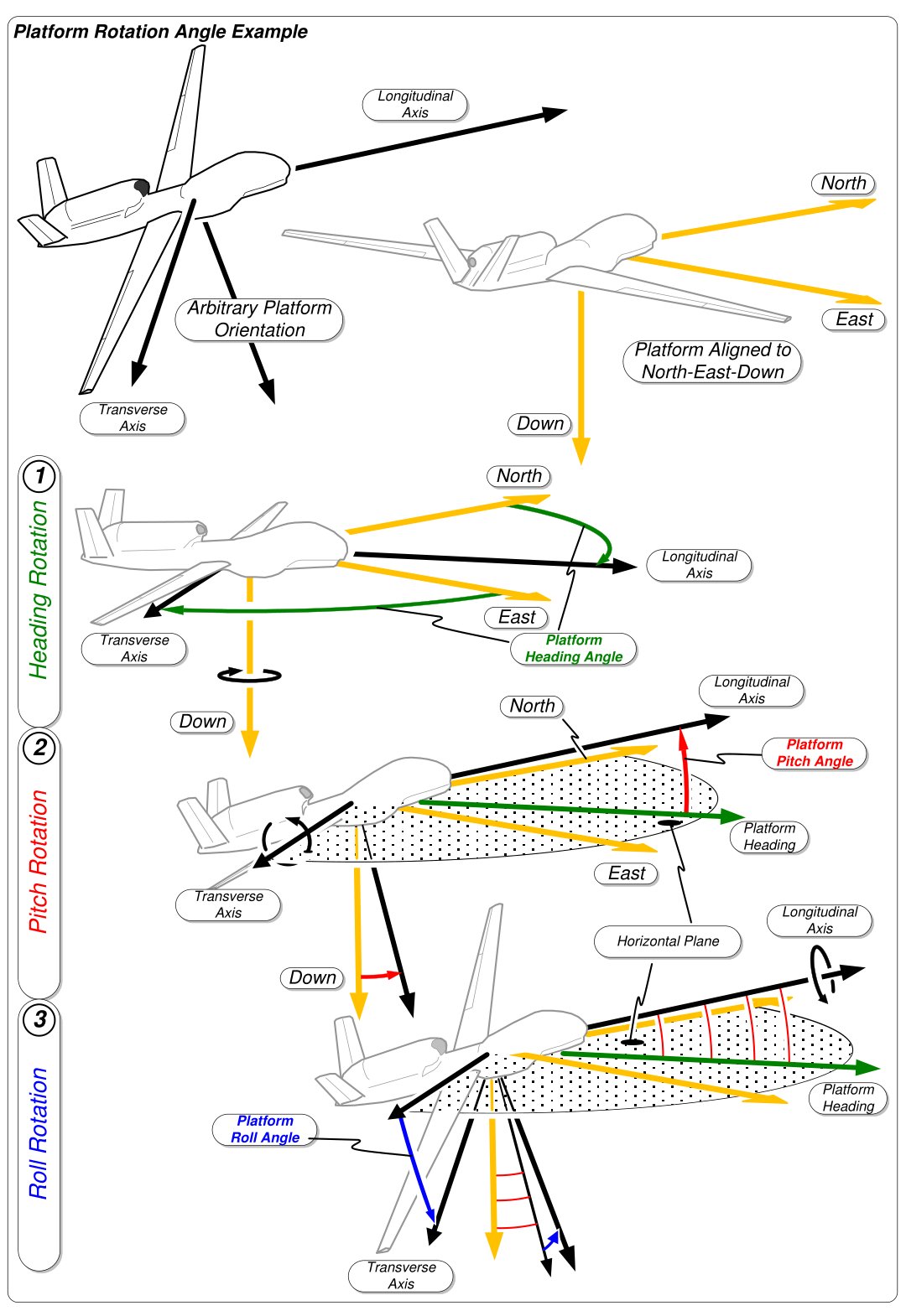
A large drone, treated as a single rigid body for navigation, has 6-DoF: three angles and three Cartesian coordinates.
Pitch, yaw (heading), and roll describe rotations about the principal axes of a drone located at point $\mathbf p = (x,y,z)^T$. Figure by the [Motion Imagery Standards Board](https://commons.wikimedia.org/wiki/File:MISB_ST_0601.8_-_Yaw,_Pitch_%26_Roll.png), public domain.
The coordinates used for the drone are one possible *configuration representation*. Other representations have different advantages and disadvantages. The drone has 6-dof when you treat its fuselage as a single rigid body and describe its configuration for navigation. For kinematic or dynamic analysis, you must also consider its many links and joints, such as the flaps, because they affect its motion. A robot generally consists of several rigid bodies whose motions are constrained by its mechanical structure. Its degrees of freedom are given by
$$
\mathrm{dof} = \text{(freedoms of the bodies)} - \text{(independent constraints)}
$$
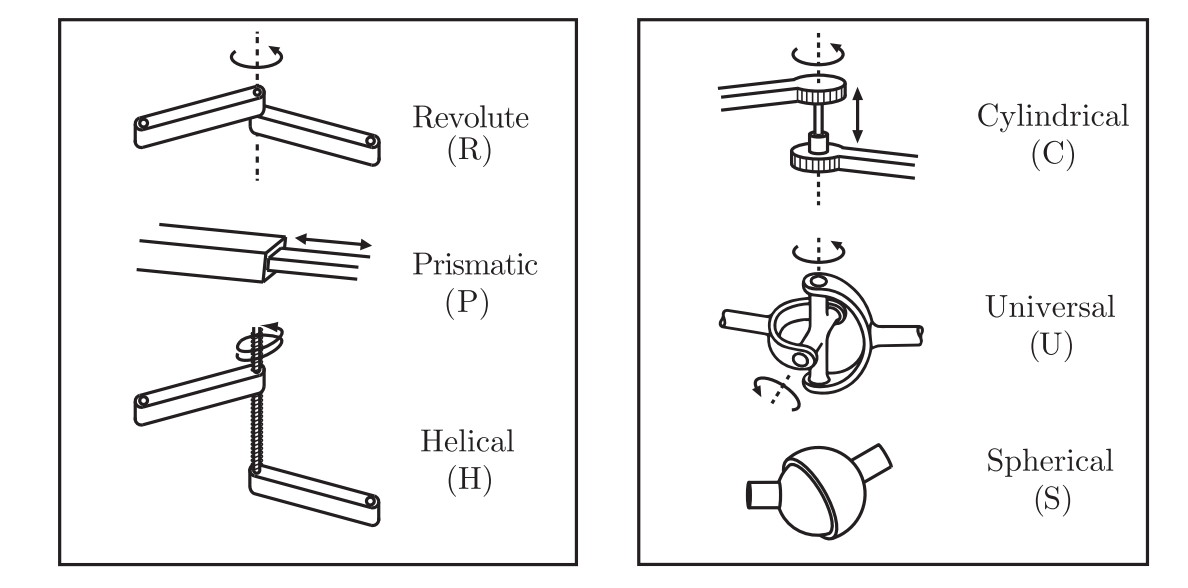
Joints constrain the motion of rigid bodies and reduce their total degrees of freedom.
The revolute joint (R), also called a hinge joint, allows rotation about the joint axis. A door commonly has three revolute joints.
The prismatic joint (P), also called a sliding or linear joint, allows translation along the joint axis. A sliding door provides a familiar example.
The helical joint (H), also called a screw joint, allows simultaneous rotation and translation about a screw axis. Revolute, prismatic,
and helical joints each have one degree of freedom.
Some joints have multiple degrees of freedom. The cylindrical joint (C) has two degrees of freedom. It allows independent translation and rotation about one fixed joint axis.
The universal joint (U) is another two-degree-of-freedom joint. It consists of two revolute joints with orthogonal
axes.
The spherical joint (S), also called a ball-and-socket
joint, has three degrees of freedom and behaves much like your shoulder joint.
The following table gives the dof of each joint when it connects planar or spatial rigid bodies.
| Joint type | DoF | Constraints between two planar rigid bodies | Constraints between two spatial rigid bodies |
| - | - | - | - |
| Revolute (R) | 1 | 2 | 5 |
| Prismatic (P) | 1 | 2 | 5 |
| Helical (H) | 1 | N/A | 5 |
| Cylindrical (C) | 2 | N/A | 4 |
| Universal (U) | 2 | N/A | 4 |
| Spherical (S) | 3 | N/A | 3 |
*Grubler's rule* gives the degrees of freedom of a robot:
$$
\mathrm{dof} = m \left( N - 1 - J \right) + \sum_{i=1}^{J} f_i
$$
where $m = 3$ for planar mechanisms and $m = 6$ for spatial mechanisms, $N$ is the number of links (including the ground link), $J$ is the number of joints, and $f_i$ is the number of degrees of freedom of joint $i$. The formula assumes that the constraints imposed by the joints are independent. When they are dependent, as can occur in closed chains, the formula gives only a lower bound on the degrees of freedom.
## Example: the human arm
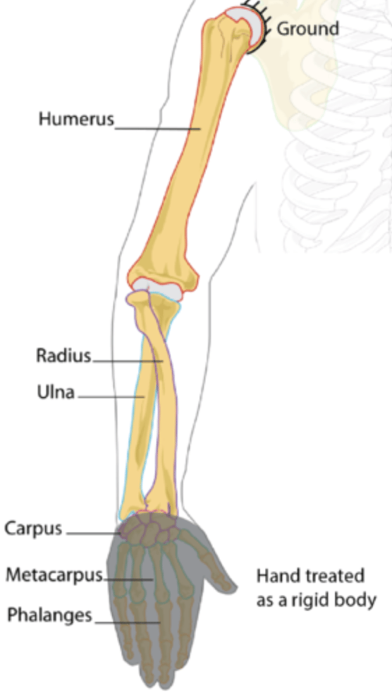
How many degrees of freedom does your arm have? Count from your torso to your palm. Keep the center of your shoulder fixed and exclude your fingers.
*The arm as a chain of four links: torso, upper arm, forearm and palm.*
Each joint of the arm corresponds to a type in the table above:
| Joint of the arm | Modeled as | dof $f$ | Constraints $c$ |
| - | - | - | - |
| Shoulder | Spherical (S) | 3 | 3 |
| Elbow and forearm | Universal (U): bending, and turning the palm up or down | 2 | 4 |
| Wrist | Universal (U): bending up and down, tilting toward the thumb or the little finger | 2 | 4 |
The four links give $N = 4$, and the three joints give $J = 3$. The joint freedoms sum to $3 + 2 + 2 = 7$. Grubler's rule with $m = 6$ gives
$$
\mathrm{dof} = 6 \left( 4 - 1 - 3 \right) + 7 = 7 .
$$
## Configuration space topology
Consider a point moving on the surface of a sphere. Its C-space
is two-dimensional because two coordinates, latitude and longitude, describe its configuration.
A point moving on a plane also has a two-dimensional C-space, with coordinates (x, y).
These spaces have different shapes. The plane extends infinitely, while the sphere wraps around.
An oval-shaped American football wraps around like a sphere. You can obtain its shape by stretching a sphere in one direction.
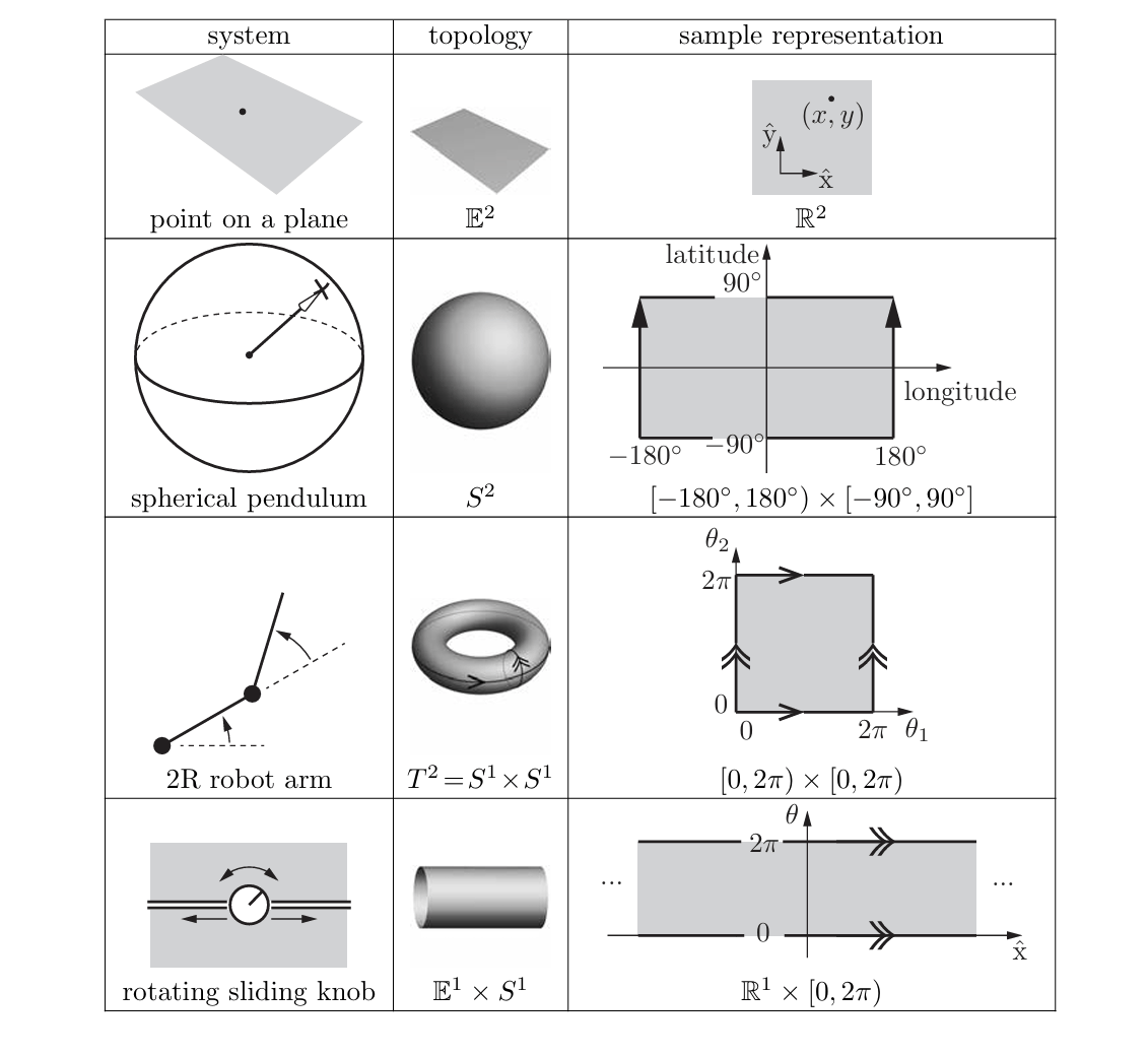
*Topology* describes the sense in which the surfaces of a small sphere, a large sphere,
and a football have the same kind of shape, while a plane has a different shape. The figure shows several example topologies.
For example, $S^2$ is the two-dimensional surface of a sphere in three-dimensional space.
The configuration space (C-space) of a rigid body in the plane is $\mathbb{R}^2 \times S^1$. The coordinates $(x, y)$ form $\mathbb{R}^2$, and the angle $\theta$ forms $S^1$.
The configuration space (C-space) of a 2R robot arm is $S^1 \times S^1 = T^2$, where $T^n$ is the $n$-dimensional surface of a torus in an $(n+1)$-dimensional space. The product $S^1 \times S^1 \times \cdots \times S^1$ (with $n$ copies of $S^1$) equals $T^n$, not $S^n$. For example, a sphere $S^2$ is not topologically equivalent to a torus $T^2$.
The topology of a space is a property of the space itself. It does not depend on the coordinates used to represent its points. You can represent a point on a circle by the angle θ from a chosen zero angle. You can instead place the origin of a reference frame at the circle's center and use two coordinates (x, y) subject to the constraint $x^2 + y^2 = 1$. The choice of coordinates does not change the space.
## C-space representation
Consider the topology of a sphere. One representation uses latitude and longitude coordinates.
A choice of $n$ coordinates, or parameters, for an n-dimensional space is called an *explicit* parametrization of
the topology of the space.
You can represent a point on the spherical surface with the coordinates used for navigation on Earth:
* Latitude (ϕ): angle from the equator (−90° at South Pole to +90° at North Pole)
* Longitude (λ): angle around the equator (from −180° to +180°)
This coordinate system works well except at the poles. Suppose you are close to the North Pole (ϕ ≈ 90°) and take a small step eastward. Your latitude ϕ changes little, but your longitude λ may change greatly. It may even jump from +180° to −180° after a small move.
A *singularity* occurs when a small physical motion causes a large coordinate change. The sphere remains smooth and uniform, so the singularity belongs to the chosen representation. Such singularities cause problems when computing velocities. Coordinate rates such as $\dot\phi$ and $\dot\lambda$ can grow very large or diverge near the poles even when the actual speed in three-dimensional space is constant.
*The point $P$ illustrates the coordinates. Longitude $\lambda$ runs around the equator from the prime meridian, while latitude $\phi$ runs from the equator toward a pole. A point then moves at constant speed along a great circle that passes 6° from the North Pole. During this pass, it crosses half the longitude range on the latitude-longitude chart, and $|\dot\lambda|$ rises sharply. The view from above explains this behavior. A small circle around the pole crosses every longitude, while the chart's entire top edge $\phi = 90^\circ$ represents the pole itself.*
The following video illustrates these problems.
You can avoid such singularities with an *implicit representation*. This representation treats an $n$-dimensional space as *embedded* in a Euclidean space of more than $n$ dimensions. For example, a two-dimensional unit sphere is a surface embedded in three-dimensional Euclidean space. An implicit representation uses the coordinates of the higher-dimensional space, such as $(x, y, z)$, with constraints that reduce the number of degrees of freedom. For the unit sphere, the constraint equation is:
$$
x^2 + y^2 + z^2 = 1
$$
This approach uses more variables than the number of degrees of freedom. It also permits linear operations, so it need not be computationally inefficient. The implicit representation given by rotation matrices encodes orientation in three-dimensional space. It uses nine numbers subject to three constraints and defines a *linear* operator.
### Velocity constraints: the TurtleBot
A configuration space describes where a robot can be. A wheeled robot cannot move in every direction from each configuration. Lynch and Park describe these limits as velocity constraints in section 2.4 (Kevin M. Lynch, 2017). A differential-drive robot such as the TurtleBot provides an example.
1. **Where can the robot be?** Its configuration is $q = (x, y, \theta)$, which gives its position in the plane and its heading. Its configuration space is $\mathbb{R}^2 \times S^1$.
2. **What motions are possible in the plane?** At a configuration $q$, the velocity $\dot q = (\dot x, \dot y, \dot\theta)$ describes an instantaneous motion. A rigid body that slides freely on a table can have any combination of these components.
3. **Which motions can the TurtleBot make?** It drives forward at speed $v$ and turns at rate $\omega$. Forward motion follows its heading, while turning changes that heading:
$$
\dot q = v \begin{bmatrix} \cos\theta \\ \sin\theta \\ 0 \end{bmatrix} + \omega \begin{bmatrix} 0 \\ 0 \\ 1 \end{bmatrix} .
$$
The first column represents forward motion, and the second represents rotation. The velocity has three components, but the robot has only these two independent choices.
4. **Which motion is forbidden?** The wheels cannot slide sideways, so the velocity perpendicular to the heading must be zero. Eliminate $v$ from $\dot x = v\cos\theta$ and $\dot y = v\sin\theta$ to obtain
$$
-\sin\theta\,\dot x + \cos\theta\,\dot y = 0, \qquad\text{that is,}\qquad A(q)\,\dot q = 0 \ \text{ with } A(q) = \begin{bmatrix} -\sin\theta & \cos\theta & 0 \end{bmatrix} .
$$
A constraint written as $A(q)\dot q = 0$ is a *Pfaffian constraint*.
5. **Does this reduce the configuration space?** No. Although the robot cannot move sideways at an instant, it can reach a point beside its starting position by turning, driving, and turning back. This velocity constraint does not limit which configurations are reachable, so you cannot integrate it into a constraint on $q$ alone. Lynch and Park call such a constraint *nonholonomic* (book pages 31 and 32).
The notation has a direct physical meaning. The vector $\dot q$ is the *configuration velocity*. All possible velocities at $q$ form the *tangent space* there. The equation $A(q)\dot q = 0$ is a *velocity constraint*. The two columns in the motion equation give the robot's *allowed directions*.
A rigid body's configuration space also has an algebraic structure. Its elements are motions that you can compose and invert. [Lie groups and tangent spaces](/aiml-common/lectures/motion-algebras/lie-theory/index) develops this structure.
### Task space
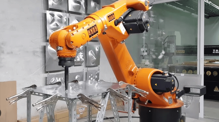
The task space is a space in which you can express the robot's task naturally. Consider incremental sheet forming, shown below. A metal sheet is clamped in a frame. The robot pushes a tool with a spherical tip into the sheet and follows a path that gradually forms the part. The path of the tip's center determines the formed surface. Rotation of the tool about that center does not change the surface. The task space is therefore $\mathbb{R}^3$, the position $(x, y, z)$ of the tip.
If the part is formed in layers of constant depth, each layer is a contour in a plane. The task space of one layer is $\mathbb{R}^2$. If the tool must tilt so that its shank does not hit the wall of a deep part, its direction becomes part of the task. The task space is then $\mathbb{R}^3 \times S^2$.
You choose the task space when describing the task, and it does not depend on the robot. A 6-dof arm performing a task in $\mathbb{R}^3$ has three degrees of freedom left. You can use them for other purposes, such as avoiding singularities or the clamping frame.
*Incremental sheet forming.*
### Workspace
The workspace specifies the end-effector configurations that the robot can reach. The robot's structure primarily determines its workspace, independently of the task.
## References
* Kevin M. Lynch, F. (2017). *Modern Robotics*.
***
Found an error on this page? [Report an issue](https://github.com/aegean-ai/eaia-feedback/issues/new?template=page-issue.yml\&page=/aiml-common/lectures/motion-algebras/configuration-space).
This documentation is built and hosted on [Mintlify](https://mintlify.com), a developer documentation platform.
 You can place the coin anywhere on the table, which gives two degrees of freedom for the $(x,y)$ coordinates. The point alone does not fix the coin's configuration. If the chosen point is Abraham Lincoln's eye, for example, the coin can still rotate through 360 degrees. The angle $\theta$ describes this additional degree of freedom.
The number of degrees of freedom (dof) of a robot is the *smallest* number of real-valued coordinates needed to represent its configuration. The discrete choice of face adds no degree of freedom. The coin has $f=3$ degrees of freedom. Its current configuration is one point in the space of all its possible configurations, called the *configuration space* (C-space).
A large drone, treated as a single rigid body for navigation, has 6-DoF: three angles and three Cartesian coordinates.
You can place the coin anywhere on the table, which gives two degrees of freedom for the $(x,y)$ coordinates. The point alone does not fix the coin's configuration. If the chosen point is Abraham Lincoln's eye, for example, the coin can still rotate through 360 degrees. The angle $\theta$ describes this additional degree of freedom.
The number of degrees of freedom (dof) of a robot is the *smallest* number of real-valued coordinates needed to represent its configuration. The discrete choice of face adds no degree of freedom. The coin has $f=3$ degrees of freedom. Its current configuration is one point in the space of all its possible configurations, called the *configuration space* (C-space).
A large drone, treated as a single rigid body for navigation, has 6-DoF: three angles and three Cartesian coordinates.
 Pitch, yaw (heading), and roll describe rotations about the principal axes of a drone located at point $\mathbf p = (x,y,z)^T$. Figure by the [Motion Imagery Standards Board](https://commons.wikimedia.org/wiki/File:MISB_ST_0601.8_-_Yaw,_Pitch_%26_Roll.png), public domain.
The coordinates used for the drone are one possible *configuration representation*. Other representations have different advantages and disadvantages. The drone has 6-dof when you treat its fuselage as a single rigid body and describe its configuration for navigation. For kinematic or dynamic analysis, you must also consider its many links and joints, such as the flaps, because they affect its motion. A robot generally consists of several rigid bodies whose motions are constrained by its mechanical structure. Its degrees of freedom are given by
$$
\mathrm{dof} = \text{(freedoms of the bodies)} - \text{(independent constraints)}
$$
Joints constrain the motion of rigid bodies and reduce their total degrees of freedom.
Pitch, yaw (heading), and roll describe rotations about the principal axes of a drone located at point $\mathbf p = (x,y,z)^T$. Figure by the [Motion Imagery Standards Board](https://commons.wikimedia.org/wiki/File:MISB_ST_0601.8_-_Yaw,_Pitch_%26_Roll.png), public domain.
The coordinates used for the drone are one possible *configuration representation*. Other representations have different advantages and disadvantages. The drone has 6-dof when you treat its fuselage as a single rigid body and describe its configuration for navigation. For kinematic or dynamic analysis, you must also consider its many links and joints, such as the flaps, because they affect its motion. A robot generally consists of several rigid bodies whose motions are constrained by its mechanical structure. Its degrees of freedom are given by
$$
\mathrm{dof} = \text{(freedoms of the bodies)} - \text{(independent constraints)}
$$
Joints constrain the motion of rigid bodies and reduce their total degrees of freedom.
 The revolute joint (R), also called a hinge joint, allows rotation about the joint axis. A door commonly has three revolute joints.
The prismatic joint (P), also called a sliding or linear joint, allows translation along the joint axis. A sliding door provides a familiar example.
The helical joint (H), also called a screw joint, allows simultaneous rotation and translation about a screw axis. Revolute, prismatic,
and helical joints each have one degree of freedom.
Some joints have multiple degrees of freedom. The cylindrical joint (C) has two degrees of freedom. It allows independent translation and rotation about one fixed joint axis.
The universal joint (U) is another two-degree-of-freedom joint. It consists of two revolute joints with orthogonal
axes.
The spherical joint (S), also called a ball-and-socket
joint, has three degrees of freedom and behaves much like your shoulder joint.
The following table gives the dof of each joint when it connects planar or spatial rigid bodies.
| Joint type | DoF | Constraints between two planar rigid bodies | Constraints between two spatial rigid bodies |
| - | - | - | - |
| Revolute (R) | 1 | 2 | 5 |
| Prismatic (P) | 1 | 2 | 5 |
| Helical (H) | 1 | N/A | 5 |
| Cylindrical (C) | 2 | N/A | 4 |
| Universal (U) | 2 | N/A | 4 |
| Spherical (S) | 3 | N/A | 3 |
*Grubler's rule* gives the degrees of freedom of a robot:
$$
\mathrm{dof} = m \left( N - 1 - J \right) + \sum_{i=1}^{J} f_i
$$
where $m = 3$ for planar mechanisms and $m = 6$ for spatial mechanisms, $N$ is the number of links (including the ground link), $J$ is the number of joints, and $f_i$ is the number of degrees of freedom of joint $i$. The formula assumes that the constraints imposed by the joints are independent. When they are dependent, as can occur in closed chains, the formula gives only a lower bound on the degrees of freedom.
## Example: the human arm
How many degrees of freedom does your arm have? Count from your torso to your palm. Keep the center of your shoulder fixed and exclude your fingers.
The revolute joint (R), also called a hinge joint, allows rotation about the joint axis. A door commonly has three revolute joints.
The prismatic joint (P), also called a sliding or linear joint, allows translation along the joint axis. A sliding door provides a familiar example.
The helical joint (H), also called a screw joint, allows simultaneous rotation and translation about a screw axis. Revolute, prismatic,
and helical joints each have one degree of freedom.
Some joints have multiple degrees of freedom. The cylindrical joint (C) has two degrees of freedom. It allows independent translation and rotation about one fixed joint axis.
The universal joint (U) is another two-degree-of-freedom joint. It consists of two revolute joints with orthogonal
axes.
The spherical joint (S), also called a ball-and-socket
joint, has three degrees of freedom and behaves much like your shoulder joint.
The following table gives the dof of each joint when it connects planar or spatial rigid bodies.
| Joint type | DoF | Constraints between two planar rigid bodies | Constraints between two spatial rigid bodies |
| - | - | - | - |
| Revolute (R) | 1 | 2 | 5 |
| Prismatic (P) | 1 | 2 | 5 |
| Helical (H) | 1 | N/A | 5 |
| Cylindrical (C) | 2 | N/A | 4 |
| Universal (U) | 2 | N/A | 4 |
| Spherical (S) | 3 | N/A | 3 |
*Grubler's rule* gives the degrees of freedom of a robot:
$$
\mathrm{dof} = m \left( N - 1 - J \right) + \sum_{i=1}^{J} f_i
$$
where $m = 3$ for planar mechanisms and $m = 6$ for spatial mechanisms, $N$ is the number of links (including the ground link), $J$ is the number of joints, and $f_i$ is the number of degrees of freedom of joint $i$. The formula assumes that the constraints imposed by the joints are independent. When they are dependent, as can occur in closed chains, the formula gives only a lower bound on the degrees of freedom.
## Example: the human arm
How many degrees of freedom does your arm have? Count from your torso to your palm. Keep the center of your shoulder fixed and exclude your fingers.
 *The arm as a chain of four links: torso, upper arm, forearm and palm.*
Each joint of the arm corresponds to a type in the table above:
| Joint of the arm | Modeled as | dof $f$ | Constraints $c$ |
| - | - | - | - |
| Shoulder | Spherical (S) | 3 | 3 |
| Elbow and forearm | Universal (U): bending, and turning the palm up or down | 2 | 4 |
| Wrist | Universal (U): bending up and down, tilting toward the thumb or the little finger | 2 | 4 |
The four links give $N = 4$, and the three joints give $J = 3$. The joint freedoms sum to $3 + 2 + 2 = 7$. Grubler's rule with $m = 6$ gives
$$
\mathrm{dof} = 6 \left( 4 - 1 - 3 \right) + 7 = 7 .
$$
## Configuration space topology
Consider a point moving on the surface of a sphere. Its C-space
is two-dimensional because two coordinates, latitude and longitude, describe its configuration.
A point moving on a plane also has a two-dimensional C-space, with coordinates (x, y).
These spaces have different shapes. The plane extends infinitely, while the sphere wraps around.
An oval-shaped American football wraps around like a sphere. You can obtain its shape by stretching a sphere in one direction.
*Topology* describes the sense in which the surfaces of a small sphere, a large sphere,
and a football have the same kind of shape, while a plane has a different shape. The figure shows several example topologies.
*The arm as a chain of four links: torso, upper arm, forearm and palm.*
Each joint of the arm corresponds to a type in the table above:
| Joint of the arm | Modeled as | dof $f$ | Constraints $c$ |
| - | - | - | - |
| Shoulder | Spherical (S) | 3 | 3 |
| Elbow and forearm | Universal (U): bending, and turning the palm up or down | 2 | 4 |
| Wrist | Universal (U): bending up and down, tilting toward the thumb or the little finger | 2 | 4 |
The four links give $N = 4$, and the three joints give $J = 3$. The joint freedoms sum to $3 + 2 + 2 = 7$. Grubler's rule with $m = 6$ gives
$$
\mathrm{dof} = 6 \left( 4 - 1 - 3 \right) + 7 = 7 .
$$
## Configuration space topology
Consider a point moving on the surface of a sphere. Its C-space
is two-dimensional because two coordinates, latitude and longitude, describe its configuration.
A point moving on a plane also has a two-dimensional C-space, with coordinates (x, y).
These spaces have different shapes. The plane extends infinitely, while the sphere wraps around.
An oval-shaped American football wraps around like a sphere. You can obtain its shape by stretching a sphere in one direction.
*Topology* describes the sense in which the surfaces of a small sphere, a large sphere,
and a football have the same kind of shape, while a plane has a different shape. The figure shows several example topologies.
 For example, $S^2$ is the two-dimensional surface of a sphere in three-dimensional space.
The configuration space (C-space) of a rigid body in the plane is $\mathbb{R}^2 \times S^1$. The coordinates $(x, y)$ form $\mathbb{R}^2$, and the angle $\theta$ forms $S^1$.
The configuration space (C-space) of a 2R robot arm is $S^1 \times S^1 = T^2$, where $T^n$ is the $n$-dimensional surface of a torus in an $(n+1)$-dimensional space. The product $S^1 \times S^1 \times \cdots \times S^1$ (with $n$ copies of $S^1$) equals $T^n$, not $S^n$. For example, a sphere $S^2$ is not topologically equivalent to a torus $T^2$.
The topology of a space is a property of the space itself. It does not depend on the coordinates used to represent its points. You can represent a point on a circle by the angle θ from a chosen zero angle. You can instead place the origin of a reference frame at the circle's center and use two coordinates (x, y) subject to the constraint $x^2 + y^2 = 1$. The choice of coordinates does not change the space.
## C-space representation
Consider the topology of a sphere. One representation uses latitude and longitude coordinates.
For example, $S^2$ is the two-dimensional surface of a sphere in three-dimensional space.
The configuration space (C-space) of a rigid body in the plane is $\mathbb{R}^2 \times S^1$. The coordinates $(x, y)$ form $\mathbb{R}^2$, and the angle $\theta$ forms $S^1$.
The configuration space (C-space) of a 2R robot arm is $S^1 \times S^1 = T^2$, where $T^n$ is the $n$-dimensional surface of a torus in an $(n+1)$-dimensional space. The product $S^1 \times S^1 \times \cdots \times S^1$ (with $n$ copies of $S^1$) equals $T^n$, not $S^n$. For example, a sphere $S^2$ is not topologically equivalent to a torus $T^2$.
The topology of a space is a property of the space itself. It does not depend on the coordinates used to represent its points. You can represent a point on a circle by the angle θ from a chosen zero angle. You can instead place the origin of a reference frame at the circle's center and use two coordinates (x, y) subject to the constraint $x^2 + y^2 = 1$. The choice of coordinates does not change the space.
## C-space representation
Consider the topology of a sphere. One representation uses latitude and longitude coordinates.
 *Incremental sheet forming.*
### Workspace
The workspace specifies the end-effector configurations that the robot can reach. The robot's structure primarily determines its workspace, independently of the task.
## References
* Kevin M. Lynch, F. (2017). *Modern Robotics*.
***
*Incremental sheet forming.*
### Workspace
The workspace specifies the end-effector configurations that the robot can reach. The robot's structure primarily determines its workspace, independently of the task.
## References
* Kevin M. Lynch, F. (2017). *Modern Robotics*.
***