> ## Documentation Index
> Fetch the complete documentation index at: https://aegean.ai/llms.txt
> Use this file to discover all available pages before exploring further.
# Homogeneous Coordinates
> Understanding homogeneous coordinates for representing points and transformations.

 *Under perspective projection, the parallel tracks appear to meet at a point on the horizon.*
A photograph maps points from three-dimensional Euclidean space to a two-dimensional image plane. Perspective projection does not preserve circles, distances, angles, or ratios of distances. A circle, for example, can appear as an ellipse. Straight lines remain straight, while parallel lines can appear to meet.
A *projective plane* extends the Euclidean plane so that every pair of distinct lines intersects in exactly one point. Parallel lines intersect at a point at infinity. In three-dimensional projective space, the same property holds for two lines in a common plane. Skew lines still do not meet (Hartley & Zisserman, 2004). A choice of coordinates selects an origin, but any point could serve as the origin.
*Under perspective projection, the parallel tracks appear to meet at a point on the horizon.*
A photograph maps points from three-dimensional Euclidean space to a two-dimensional image plane. Perspective projection does not preserve circles, distances, angles, or ratios of distances. A circle, for example, can appear as an ellipse. Straight lines remain straight, while parallel lines can appear to meet.
A *projective plane* extends the Euclidean plane so that every pair of distinct lines intersects in exactly one point. Parallel lines intersect at a point at infinity. In three-dimensional projective space, the same property holds for two lines in a common plane. Skew lines still do not meet (Hartley & Zisserman, 2004). A choice of coordinates selects an origin, but any point could serve as the origin.
 *The coordinates of a point in 2D depend on the chosen coordinate system. The solid and dashed axes define two coordinate systems, so the same point has different coordinates in each. Its position in space does not change.*
The figure shows two *frames*. Each frame consists of an origin and two linearly independent basis vectors that define the axes of the two-dimensional space. More generally, an origin $p_o$ and $n$ linearly independent basis vectors define an n-dimensional *affine frame*. For any vector $\mathbf v$, a unique set of scalars $s_i$ satisfies
$\mathbf v = s_1 \mathbf u_1 + s_2 \mathbf u_2 + ... + s_n \mathbf u_n = \mathbf s^T [\mathbf u_1, \mathbf u_2, ..., \mathbf u_n]^T $
where $\mathbf s$ gives the coordinates of $\mathbf v$ in the frame. Each point also has unique scalars $s_i$ that express it in terms of the origin $p_o$ and the basis vectors:
$p = p_o + s_1 \mathbf u_1 + s_2 \mathbf u_2 + ... + s_n \mathbf u_n = p_o + \mathbf s^T [\mathbf u_1, \mathbf u_2, ..., \mathbf u_n]^T$
An affine space of dimension $n$ consists of a set of points $\mathcal{A}$ and an associated vector space $V$ of dimension $n$. It supports two operations:
* Point subtraction: $p - q \in V$ (gives a vector)
* Point translation: $p + v \in \mathcal{A}$ (moves a point by a vector)
An affine space has no fixed origin, preferred coordinate system, or basis until you choose one.
A coordinate frame on an affine space consists of a chosen origin point $p_0 \in \mathcal{A}$ and a basis $\{v_1, \dots, v_n\}$ for the associated vector space $V$.
A vector space has a built-in origin, defined by the zero vector. It is closed under addition and scalar multiplication, so it supports linear combinations such as $a\mathbf{v}_1 + b\mathbf{v}_2$. For this reason, it is also called a linear space. In an affine space, you cannot add two points directly, and there is no zero point.
Euclidean space adds an inner product, which defines angles and lengths.
Points and vectors may both have x, y, and z coordinates in 3D, but they are different mathematical objects. A 3D frame defined by $(p_o, \mathbf u_1, \mathbf u_2, \mathbf u_3)$ does not distinguish a point $(p_x, p_y, p_z)$ from a vector $(v_x, v_y, v_z)$ with the same coordinates. Homogeneous coordinates make the distinction explicit. In this frame, the point is
$p = [s_1 s_2 s_3 1][\mathbf u_1 \mathbf u_2 \mathbf u_3 p_o]^T$
and the vector is
$\mathbf v = [s_1' s_2' s_3' 0][\mathbf u_1 \mathbf u_2 \mathbf u_3 p_o]^T$
The point representation $[s_1 s_2 s_3 1]$ and the vector representation $[s_1' s_2' s_3' 0]$ are called *homogeneous coordinates*. The fourth coordinate $w$ is the *weight*. A point $(x,y,z)$ in three-dimensional Euclidean space can be represented by the 4-tuple $(x,y,z,1)$. More generally, $(x,y,z,1)$ and $(\lambda x, \lambda y, \lambda z, \lambda)$ represent the same point for any $\lambda \neq 0$. Dividing every coordinate by $\lambda$ gives $(x,y,z,1)$. A point with weight $w \neq 0$ therefore represents the Cartesian point obtained by dividing by the weight:
$(x, y, z, w) \equiv (x/w,\; y/w,\; z/w), \qquad w \neq 0$
Homogeneous coordinates represent a family of equivalent points along a ray in projective space. Each member is a scaled version of the same Cartesian point. These coordinates can:
* Represent points at infinity (when $w = 0$), as required for parallel lines in perspective projections.
* Express transformations such as perspective camera models and 3D projections as linear matrix operations.
## Transformations in homogeneous coordinates
Homogeneous matrices represent common 2D transformations.
### Rigid transformation
A rigid transformation combines a rotation and a translation. It preserves lengths and angles and does not include scaling or shearing.
Its matrix is
$$
\mathbf{T}_{\text{rigid}} =
\begin{bmatrix}
\cos\theta & -\sin\theta & t_x \\
\sin\theta & \cos\theta & t_y \\
0 & 0 & 1
\end{bmatrix}
$$
* $\theta$: rotation angle
* $(t_x, t_y)$: translation
### Similarity transformation
A similarity transformation includes rotation, translation, and uniform scaling. It preserves shape but not necessarily size.
$$
\mathbf{T}_{\text{sim}} =
\begin{bmatrix}
s \cos\theta & -s \sin\theta & t_x \\
s \sin\theta & s \cos\theta & t_y \\
0 & 0 & 1
\end{bmatrix}
$$
The scaling factor is $s$.
### Affine transformation
An affine transformation can combine translation, rotation, scaling, and shearing. It preserves parallel lines, but it need not preserve lengths or angles.
$$
\mathbf{T}_{\text{affine}} =
\begin{bmatrix}
a_{11} & a_{12} & t_x \\
a_{21} & a_{22} & t_y \\
0 & 0 & 1
\end{bmatrix}
$$
This matrix gives the general form of a 2D affine transformation.
## Example
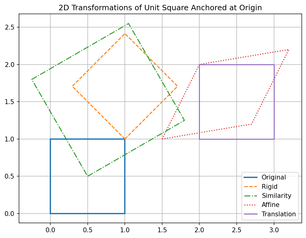
The following code applies each transformation to a square:
```python theme={null}
import matplotlib.pyplot as plt
import numpy as np
# Original square: corner at origin, size 1
square = np.array(
[
[0, 0, 1],
[1, 0, 1],
[1, 1, 1],
[0, 1, 1],
[0, 0, 1], # close the square
]
).T
# Define transformations
def apply_transform(matrix, shape):
return (matrix @ shape).T[:, :2]
# Rigid: rotate 45 deg and translate (1, 1)
theta = np.pi / 4
T_rigid = np.array(
[[np.cos(theta), -np.sin(theta), 1], [np.sin(theta), np.cos(theta), 1], [0, 0, 1]]
)
# Similarity: scale by 1.5, rotate 30 deg, translate (0.5, 0.5)
theta_sim = np.pi / 6
s = 1.5
T_similarity = np.array(
[
[s * np.cos(theta_sim), -s * np.sin(theta_sim), 0.5],
[s * np.sin(theta_sim), s * np.cos(theta_sim), 0.5],
[0, 0, 1],
]
)
# Affine: shear and scale
T_affine = np.array([[1.2, 0.5, 1.5], [0.2, 1.0, 1.0], [0, 0, 1]])
# Translation only
T_translation = np.array([[1, 0, 2], [0, 1, 1], [0, 0, 1]])
# Apply transformations
square_rigid = apply_transform(T_rigid, square)
square_similarity = apply_transform(T_similarity, square)
square_affine = apply_transform(T_affine, square)
square_translation = apply_transform(T_translation, square)
square_original = square.T[:, :2]
```
*The coordinates of a point in 2D depend on the chosen coordinate system. The solid and dashed axes define two coordinate systems, so the same point has different coordinates in each. Its position in space does not change.*
The figure shows two *frames*. Each frame consists of an origin and two linearly independent basis vectors that define the axes of the two-dimensional space. More generally, an origin $p_o$ and $n$ linearly independent basis vectors define an n-dimensional *affine frame*. For any vector $\mathbf v$, a unique set of scalars $s_i$ satisfies
$\mathbf v = s_1 \mathbf u_1 + s_2 \mathbf u_2 + ... + s_n \mathbf u_n = \mathbf s^T [\mathbf u_1, \mathbf u_2, ..., \mathbf u_n]^T $
where $\mathbf s$ gives the coordinates of $\mathbf v$ in the frame. Each point also has unique scalars $s_i$ that express it in terms of the origin $p_o$ and the basis vectors:
$p = p_o + s_1 \mathbf u_1 + s_2 \mathbf u_2 + ... + s_n \mathbf u_n = p_o + \mathbf s^T [\mathbf u_1, \mathbf u_2, ..., \mathbf u_n]^T$
An affine space of dimension $n$ consists of a set of points $\mathcal{A}$ and an associated vector space $V$ of dimension $n$. It supports two operations:
* Point subtraction: $p - q \in V$ (gives a vector)
* Point translation: $p + v \in \mathcal{A}$ (moves a point by a vector)
An affine space has no fixed origin, preferred coordinate system, or basis until you choose one.
A coordinate frame on an affine space consists of a chosen origin point $p_0 \in \mathcal{A}$ and a basis $\{v_1, \dots, v_n\}$ for the associated vector space $V$.
A vector space has a built-in origin, defined by the zero vector. It is closed under addition and scalar multiplication, so it supports linear combinations such as $a\mathbf{v}_1 + b\mathbf{v}_2$. For this reason, it is also called a linear space. In an affine space, you cannot add two points directly, and there is no zero point.
Euclidean space adds an inner product, which defines angles and lengths.
Points and vectors may both have x, y, and z coordinates in 3D, but they are different mathematical objects. A 3D frame defined by $(p_o, \mathbf u_1, \mathbf u_2, \mathbf u_3)$ does not distinguish a point $(p_x, p_y, p_z)$ from a vector $(v_x, v_y, v_z)$ with the same coordinates. Homogeneous coordinates make the distinction explicit. In this frame, the point is
$p = [s_1 s_2 s_3 1][\mathbf u_1 \mathbf u_2 \mathbf u_3 p_o]^T$
and the vector is
$\mathbf v = [s_1' s_2' s_3' 0][\mathbf u_1 \mathbf u_2 \mathbf u_3 p_o]^T$
The point representation $[s_1 s_2 s_3 1]$ and the vector representation $[s_1' s_2' s_3' 0]$ are called *homogeneous coordinates*. The fourth coordinate $w$ is the *weight*. A point $(x,y,z)$ in three-dimensional Euclidean space can be represented by the 4-tuple $(x,y,z,1)$. More generally, $(x,y,z,1)$ and $(\lambda x, \lambda y, \lambda z, \lambda)$ represent the same point for any $\lambda \neq 0$. Dividing every coordinate by $\lambda$ gives $(x,y,z,1)$. A point with weight $w \neq 0$ therefore represents the Cartesian point obtained by dividing by the weight:
$(x, y, z, w) \equiv (x/w,\; y/w,\; z/w), \qquad w \neq 0$
Homogeneous coordinates represent a family of equivalent points along a ray in projective space. Each member is a scaled version of the same Cartesian point. These coordinates can:
* Represent points at infinity (when $w = 0$), as required for parallel lines in perspective projections.
* Express transformations such as perspective camera models and 3D projections as linear matrix operations.
## Transformations in homogeneous coordinates
Homogeneous matrices represent common 2D transformations.
### Rigid transformation
A rigid transformation combines a rotation and a translation. It preserves lengths and angles and does not include scaling or shearing.
Its matrix is
$$
\mathbf{T}_{\text{rigid}} =
\begin{bmatrix}
\cos\theta & -\sin\theta & t_x \\
\sin\theta & \cos\theta & t_y \\
0 & 0 & 1
\end{bmatrix}
$$
* $\theta$: rotation angle
* $(t_x, t_y)$: translation
### Similarity transformation
A similarity transformation includes rotation, translation, and uniform scaling. It preserves shape but not necessarily size.
$$
\mathbf{T}_{\text{sim}} =
\begin{bmatrix}
s \cos\theta & -s \sin\theta & t_x \\
s \sin\theta & s \cos\theta & t_y \\
0 & 0 & 1
\end{bmatrix}
$$
The scaling factor is $s$.
### Affine transformation
An affine transformation can combine translation, rotation, scaling, and shearing. It preserves parallel lines, but it need not preserve lengths or angles.
$$
\mathbf{T}_{\text{affine}} =
\begin{bmatrix}
a_{11} & a_{12} & t_x \\
a_{21} & a_{22} & t_y \\
0 & 0 & 1
\end{bmatrix}
$$
This matrix gives the general form of a 2D affine transformation.
## Example
The following code applies each transformation to a square:
```python theme={null}
import matplotlib.pyplot as plt
import numpy as np
# Original square: corner at origin, size 1
square = np.array(
[
[0, 0, 1],
[1, 0, 1],
[1, 1, 1],
[0, 1, 1],
[0, 0, 1], # close the square
]
).T
# Define transformations
def apply_transform(matrix, shape):
return (matrix @ shape).T[:, :2]
# Rigid: rotate 45 deg and translate (1, 1)
theta = np.pi / 4
T_rigid = np.array(
[[np.cos(theta), -np.sin(theta), 1], [np.sin(theta), np.cos(theta), 1], [0, 0, 1]]
)
# Similarity: scale by 1.5, rotate 30 deg, translate (0.5, 0.5)
theta_sim = np.pi / 6
s = 1.5
T_similarity = np.array(
[
[s * np.cos(theta_sim), -s * np.sin(theta_sim), 0.5],
[s * np.sin(theta_sim), s * np.cos(theta_sim), 0.5],
[0, 0, 1],
]
)
# Affine: shear and scale
T_affine = np.array([[1.2, 0.5, 1.5], [0.2, 1.0, 1.0], [0, 0, 1]])
# Translation only
T_translation = np.array([[1, 0, 2], [0, 1, 1], [0, 0, 1]])
# Apply transformations
square_rigid = apply_transform(T_rigid, square)
square_similarity = apply_transform(T_similarity, square)
square_affine = apply_transform(T_affine, square)
square_translation = apply_transform(T_translation, square)
square_original = square.T[:, :2]
```
 ## References
* Hartley, R., Zisserman, A. (2004). *Multiple View Geometry in Computer Vision*.
***
Found an error on this page? [Report an issue](https://github.com/aegean-ai/eaia-feedback/issues/new?template=page-issue.yml\&page=/aiml-common/lectures/motion-algebras/homogeneous-coordinates).
This documentation is built and hosted on [Mintlify](https://mintlify.com), a developer documentation platform.
## References
* Hartley, R., Zisserman, A. (2004). *Multiple View Geometry in Computer Vision*.
***
Found an error on this page? [Report an issue](https://github.com/aegean-ai/eaia-feedback/issues/new?template=page-issue.yml\&page=/aiml-common/lectures/motion-algebras/homogeneous-coordinates).
This documentation is built and hosted on [Mintlify](https://mintlify.com), a developer documentation platform.