> ## Documentation Index
> Fetch the complete documentation index at: https://aegean.ai/llms.txt
> Use this file to discover all available pages before exploring further.
# The rotation group SO(2) as a circle
> How 2x2 rotation matrices trace a one-dimensional circle inside four-dimensional matrix space as the angle changes.
 A $2 \times 2$ matrix has four entries, so you can view it as a point in $\mathbb{R}^4$. Most of these points are not rotations. A rotation matrix must satisfy three constraints: each column has unit length (two constraints), and the columns are orthogonal (one constraint). Four entries minus three constraints leaves one degree of freedom, the angle $\theta$.
$$
R(\theta) = \begin{bmatrix} \cos\theta & -\sin\theta \\ \sin\theta & \cos\theta \end{bmatrix}
$$
As $\theta$ changes, $R(\theta)$ traces a curve in $\mathbb{R}^4$. That curve is $SO(2)$, a one-dimensional manifold inside a four-dimensional space. The calculations and figures below construct this curve, determine its shape, and relate its velocity to an element of $\mathfrak{so}(2)$.
This section studies $SO(2)$ and its Lie algebra $\mathfrak{so}(2)$, the first two rows of the table in the [Lie cheatsheet](/aiml-common/lectures/motion-algebras/lie-cheatsheet/index). Their geometry can be computed and drawn directly.
## Sampling the curve
Each value of $\theta$ gives one rotation matrix. Flattening the matrix row by row gives a point in $\mathbb{R}^4$ with coordinates $(r_{11}, r_{12}, r_{21}, r_{22})$.
```python theme={null}
import matplotlib.pyplot as plt
import numpy as np
def rot(theta):
c, s = np.cos(theta), np.sin(theta)
return np.array([[c, -s], [s, c]])
thetas = np.linspace(0, 2 * np.pi, 400)
Rs = np.stack([rot(t) for t in thetas]) # shape (400, 2, 2)
points = Rs.reshape(len(thetas), 4) # (r11, r12, r21, r22) per row
# Every sample satisfies the rotation constraints
orth_err = np.abs(np.einsum("nji,njk->nik", Rs, Rs) - np.eye(2)).max()
det_err = np.abs(np.linalg.det(Rs) - 1).max()
print(f"max |R^T R - I| = {orth_err:.1e}")
print(f"max |det R - 1| = {det_err:.1e}")
```
```output theme={null}
max |R^T R - I| = 2.2e-16
max |det R - 1| = 2.2e-16
```
## The shape of the curve
The four coordinates of $R(\theta)$ are $(\cos\theta, -\sin\theta, \sin\theta, \cos\theta)$. They satisfy two linear relations: $r_{22} = r_{11}$ and $r_{12} = -r_{21}$. These relations confine the curve to a two-dimensional plane inside $\mathbb{R}^4$. Within that plane, the remaining constraint $r_{11}^2 + r_{21}^2 = 1$ is the equation of a circle.
Thus $SO(2)$ is a circle. Its distance from the origin of $\mathbb{R}^4$ is the Frobenius norm of $R$, which is $\sqrt{2}$ for every rotation. The curve is closed because $\theta$ and $\theta + 2\pi$ give the same matrix. The calculation below checks the two linear relations and the distance from the origin.
```python theme={null}
r11, r12, r21, r22 = points.T
print(f"max |r22 - r11| = {np.abs(r22 - r11).max():.1e}")
print(f"max |r12 + r21| = {np.abs(r12 + r21).max():.1e}")
print(f"distance from origin = {np.linalg.norm(points, axis=1).min():.4f} to {np.linalg.norm(points, axis=1).max():.4f}")
print(f"sqrt(2) = {np.sqrt(2):.4f}")
print(f"closes on itself = {np.allclose(rot(0), rot(2 * np.pi))}")
```
```output theme={null}
max |r22 - r11| = 0.0e+00
max |r12 + r21| = 0.0e+00
distance from origin = 1.4142 to 1.4142
sqrt(2) = 1.4142
closes on itself = True
```
## Drawing the curve
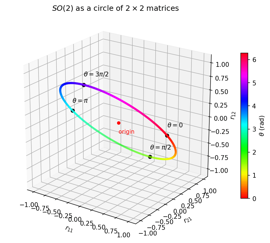
You cannot draw $\mathbb{R}^4$, but the relations among the entries let you use fewer coordinates. Because $r_{22}$ always equals $r_{11}$, dropping it loses no information. The plot below uses the three coordinates $(r_{11}, r_{21}, r_{12})$, and color indicates the angle $\theta$. The curve is a tilted circle centered at the origin.
A $2 \times 2$ matrix has four entries, so you can view it as a point in $\mathbb{R}^4$. Most of these points are not rotations. A rotation matrix must satisfy three constraints: each column has unit length (two constraints), and the columns are orthogonal (one constraint). Four entries minus three constraints leaves one degree of freedom, the angle $\theta$.
$$
R(\theta) = \begin{bmatrix} \cos\theta & -\sin\theta \\ \sin\theta & \cos\theta \end{bmatrix}
$$
As $\theta$ changes, $R(\theta)$ traces a curve in $\mathbb{R}^4$. That curve is $SO(2)$, a one-dimensional manifold inside a four-dimensional space. The calculations and figures below construct this curve, determine its shape, and relate its velocity to an element of $\mathfrak{so}(2)$.
This section studies $SO(2)$ and its Lie algebra $\mathfrak{so}(2)$, the first two rows of the table in the [Lie cheatsheet](/aiml-common/lectures/motion-algebras/lie-cheatsheet/index). Their geometry can be computed and drawn directly.
## Sampling the curve
Each value of $\theta$ gives one rotation matrix. Flattening the matrix row by row gives a point in $\mathbb{R}^4$ with coordinates $(r_{11}, r_{12}, r_{21}, r_{22})$.
```python theme={null}
import matplotlib.pyplot as plt
import numpy as np
def rot(theta):
c, s = np.cos(theta), np.sin(theta)
return np.array([[c, -s], [s, c]])
thetas = np.linspace(0, 2 * np.pi, 400)
Rs = np.stack([rot(t) for t in thetas]) # shape (400, 2, 2)
points = Rs.reshape(len(thetas), 4) # (r11, r12, r21, r22) per row
# Every sample satisfies the rotation constraints
orth_err = np.abs(np.einsum("nji,njk->nik", Rs, Rs) - np.eye(2)).max()
det_err = np.abs(np.linalg.det(Rs) - 1).max()
print(f"max |R^T R - I| = {orth_err:.1e}")
print(f"max |det R - 1| = {det_err:.1e}")
```
```output theme={null}
max |R^T R - I| = 2.2e-16
max |det R - 1| = 2.2e-16
```
## The shape of the curve
The four coordinates of $R(\theta)$ are $(\cos\theta, -\sin\theta, \sin\theta, \cos\theta)$. They satisfy two linear relations: $r_{22} = r_{11}$ and $r_{12} = -r_{21}$. These relations confine the curve to a two-dimensional plane inside $\mathbb{R}^4$. Within that plane, the remaining constraint $r_{11}^2 + r_{21}^2 = 1$ is the equation of a circle.
Thus $SO(2)$ is a circle. Its distance from the origin of $\mathbb{R}^4$ is the Frobenius norm of $R$, which is $\sqrt{2}$ for every rotation. The curve is closed because $\theta$ and $\theta + 2\pi$ give the same matrix. The calculation below checks the two linear relations and the distance from the origin.
```python theme={null}
r11, r12, r21, r22 = points.T
print(f"max |r22 - r11| = {np.abs(r22 - r11).max():.1e}")
print(f"max |r12 + r21| = {np.abs(r12 + r21).max():.1e}")
print(f"distance from origin = {np.linalg.norm(points, axis=1).min():.4f} to {np.linalg.norm(points, axis=1).max():.4f}")
print(f"sqrt(2) = {np.sqrt(2):.4f}")
print(f"closes on itself = {np.allclose(rot(0), rot(2 * np.pi))}")
```
```output theme={null}
max |r22 - r11| = 0.0e+00
max |r12 + r21| = 0.0e+00
distance from origin = 1.4142 to 1.4142
sqrt(2) = 1.4142
closes on itself = True
```
## Drawing the curve
You cannot draw $\mathbb{R}^4$, but the relations among the entries let you use fewer coordinates. Because $r_{22}$ always equals $r_{11}$, dropping it loses no information. The plot below uses the three coordinates $(r_{11}, r_{21}, r_{12})$, and color indicates the angle $\theta$. The curve is a tilted circle centered at the origin.
 **The determinant as signed area**
The *unit square* has corners $(0,0)$, $(1,0)$, $(1,1)$ and $(0,1)$. Its sides are the basis vectors $\mathbf{e}_1 = (1, 0)$ and $\mathbf{e}_2 = (0, 1)$, and its area is 1. A matrix sends $\mathbf{e}_1$ to its first column and $\mathbf{e}_2$ to its second column. It therefore sends the unit square to the parallelogram spanned by its columns. For
$$
A = \begin{bmatrix} a & b \\ c & d \end{bmatrix}
$$
that parallelogram has signed area $ad - bc$, which is $\det A$. Since the original square has area 1, the determinant is the factor by which the matrix scales area. The same factor applies to every region because any region can be tiled with small squares.
The sign records orientation. Walking around the unit square from $\mathbf{e}_1$ to $\mathbf{e}_2$ is a counterclockwise turn. The determinant is positive if the image of $\mathbf{e}_2$ remains counterclockwise from the image of $\mathbf{e}_1$. If the matrix reflects the square, that turn becomes clockwise and the determinant is negative. A determinant of zero means that the square is flattened onto a line and the matrix cannot be undone.
The determinant does not measure the size of a matrix. $\begin{bmatrix} 3 & 0 \\ 0 & 1/3 \end{bmatrix}$ stretches one direction by a factor of 3, yet its determinant is 1 because the squeeze in the other direction preserves area. A matrix's effect on vector lengths is measured by its norm or singular values. The calculations and plots below compare these cases.
```python theme={null}
examples = {
"rotation by 30°": rot(np.pi / 6),
"reflection": np.array([[np.cos(np.pi / 3), np.sin(np.pi / 3)], [np.sin(np.pi / 3), -np.cos(np.pi / 3)]]),
"uniform scaling by 1.5": 1.5 * np.eye(2),
"stretch and squeeze": np.array([[3, 0], [0, 1 / 3]]),
"singular": np.array([[1, 0.5], [1, 0.5]]),
}
unit_square = np.array([[0, 0], [1, 0], [1, 1], [0, 1]]).T # corners as columns
def signed_area(corners):
# Shoelace formula; corners has shape (2, N) in walking order
x, y = corners
return 0.5 * np.sum(x * np.roll(y, -1) - np.roll(x, -1) * y)
for name, A in examples.items():
image = A @ unit_square
print(f"{name:24s} det = {np.linalg.det(A):+.3f} signed area of image = {signed_area(image):+.3f}")
```
```output theme={null}
rotation by 30° det = +1.000 signed area of image = +1.000
reflection det = -1.000 signed area of image = -1.000
uniform scaling by 1.5 det = +2.250 signed area of image = +2.250
stretch and squeeze det = +1.000 signed area of image = +1.000
singular det = +0.000 signed area of image = +0.000
```
**The determinant as signed area**
The *unit square* has corners $(0,0)$, $(1,0)$, $(1,1)$ and $(0,1)$. Its sides are the basis vectors $\mathbf{e}_1 = (1, 0)$ and $\mathbf{e}_2 = (0, 1)$, and its area is 1. A matrix sends $\mathbf{e}_1$ to its first column and $\mathbf{e}_2$ to its second column. It therefore sends the unit square to the parallelogram spanned by its columns. For
$$
A = \begin{bmatrix} a & b \\ c & d \end{bmatrix}
$$
that parallelogram has signed area $ad - bc$, which is $\det A$. Since the original square has area 1, the determinant is the factor by which the matrix scales area. The same factor applies to every region because any region can be tiled with small squares.
The sign records orientation. Walking around the unit square from $\mathbf{e}_1$ to $\mathbf{e}_2$ is a counterclockwise turn. The determinant is positive if the image of $\mathbf{e}_2$ remains counterclockwise from the image of $\mathbf{e}_1$. If the matrix reflects the square, that turn becomes clockwise and the determinant is negative. A determinant of zero means that the square is flattened onto a line and the matrix cannot be undone.
The determinant does not measure the size of a matrix. $\begin{bmatrix} 3 & 0 \\ 0 & 1/3 \end{bmatrix}$ stretches one direction by a factor of 3, yet its determinant is 1 because the squeeze in the other direction preserves area. A matrix's effect on vector lengths is measured by its norm or singular values. The calculations and plots below compare these cases.
```python theme={null}
examples = {
"rotation by 30°": rot(np.pi / 6),
"reflection": np.array([[np.cos(np.pi / 3), np.sin(np.pi / 3)], [np.sin(np.pi / 3), -np.cos(np.pi / 3)]]),
"uniform scaling by 1.5": 1.5 * np.eye(2),
"stretch and squeeze": np.array([[3, 0], [0, 1 / 3]]),
"singular": np.array([[1, 0.5], [1, 0.5]]),
}
unit_square = np.array([[0, 0], [1, 0], [1, 1], [0, 1]]).T # corners as columns
def signed_area(corners):
# Shoelace formula; corners has shape (2, N) in walking order
x, y = corners
return 0.5 * np.sum(x * np.roll(y, -1) - np.roll(x, -1) * y)
for name, A in examples.items():
image = A @ unit_square
print(f"{name:24s} det = {np.linalg.det(A):+.3f} signed area of image = {signed_area(image):+.3f}")
```
```output theme={null}
rotation by 30° det = +1.000 signed area of image = +1.000
reflection det = -1.000 signed area of image = -1.000
uniform scaling by 1.5 det = +2.250 signed area of image = +2.250
stretch and squeeze det = +1.000 signed area of image = +1.000
singular det = +0.000 signed area of image = +0.000
```
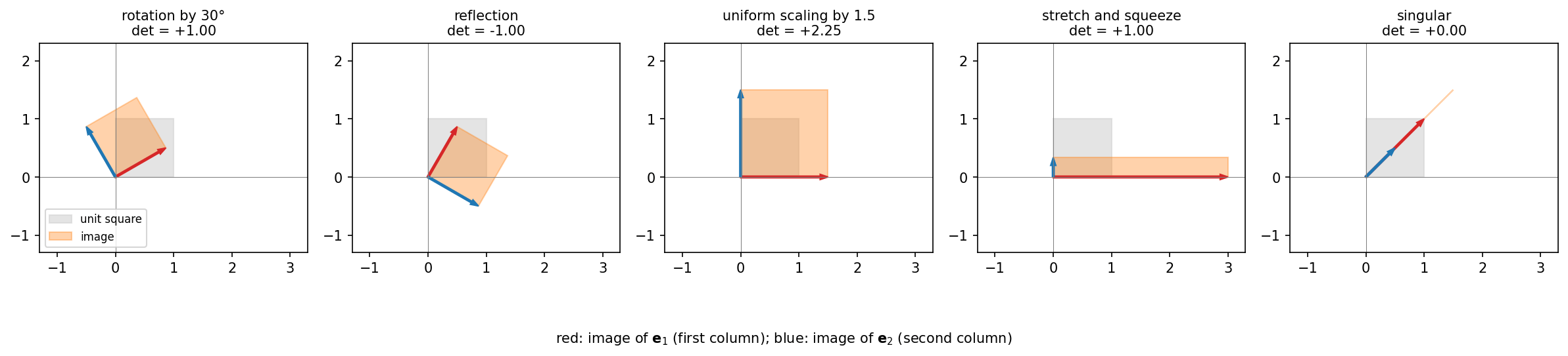 In the rotation, the red and blue arrows keep their counterclockwise order, and the square keeps its area. In the reflection, the area is unchanged, but the blue arrow is clockwise from the red one. The uniform scaling multiplies the area by $1.5^2 = 2.25$. The stretch and squeeze map changes the shape but preserves the area. The singular matrix sends both columns onto the same line, so the square has no area left.
## Rotations and reflections
Orthonormal columns alone do not make a rotation. The matrices
$$
F(\theta) = \begin{bmatrix} \cos\theta & \sin\theta \\ \sin\theta & -\cos\theta \end{bmatrix}
$$
also have orthonormal columns, but $\det F = -1$. Each is a reflection across a line through the origin. As $\theta$ changes, these matrices trace a second circle in $\mathbb{R}^4$. The two circles together form $O(2)$, the group of all orthogonal $2 \times 2$ matrices. The condition $\det R = +1$ selects the circle containing the identity.
No continuous path of orthogonal matrices can turn a rotation into a reflection because $\det$ would have to jump from $+1$ to $-1$. Thus $SO(2)$ is a manifold in its own right. The calculation below confirms that every rotation is at distance 2 from every reflection.
```python theme={null}
def refl(theta):
c, s = np.cos(theta), np.sin(theta)
return np.array([[c, s], [s, -c]])
Fs = np.stack([refl(t) for t in thetas])
print(f"det of reflections: {np.linalg.det(Fs).min():.3f} to {np.linalg.det(Fs).max():.3f}")
# Distance in R^4 between every rotation and every reflection
F_points = Fs.reshape(len(thetas), 4)
dists = np.linalg.norm(points[:, None, :] - F_points[None, :, :], axis=2)
print(f"rotation-to-reflection distance: min {dists.min():.4f}, max {dists.max():.4f}")
```
```output theme={null}
det of reflections: -1.000 to -1.000
rotation-to-reflection distance: min 2.0000, max 2.0000
```
## Seeing both circles
The coordinates $(r_{11}, r_{12}, r_{21}, r_{22})$ hide the geometry. The relations satisfied by each family suggest another set of axes for $\mathbb{R}^4$:
$$
a = \tfrac{r_{11} + r_{22}}{\sqrt{2}}, \quad
b = \tfrac{r_{21} - r_{12}}{\sqrt{2}}, \quad
c = \tfrac{r_{11} - r_{22}}{\sqrt{2}}, \quad
d = \tfrac{r_{21} + r_{12}}{\sqrt{2}}
$$
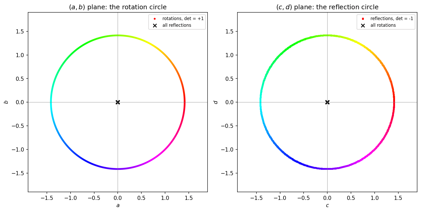
These four axes are orthonormal, so they describe the same space without distortion. A rotation has $c = d = 0$ and lands at $(a, b) = \sqrt{2}(\cos\theta, \sin\theta)$. A reflection has $a = b = 0$ and lands at $(c, d) = \sqrt{2}(\cos\theta, \sin\theta)$. Thus $\mathbb{R}^4$ splits into two perpendicular planes. The rotations form a circle of radius $\sqrt{2}$ in the $(a, b)$ plane. The reflections form a circle of the same radius in the $(c, d)$ plane.
Each circle projects to the origin of the other plane. This also explains the constant distance. Any rotation is $\sqrt{2}$ from the origin in one plane, and any reflection is $\sqrt{2}$ from the origin in the perpendicular plane. By Pythagoras, they are $\sqrt{2 + 2} = 2$ apart. The calculation and plots below show this decomposition.
```python theme={null}
def plane_coords(M):
# M has shape (N, 2, 2); returns (N, 4) with columns a, b, c, d
r11, r12, r21, r22 = M[:, 0, 0], M[:, 0, 1], M[:, 1, 0], M[:, 1, 1]
return np.stack([r11 + r22, r21 - r12, r11 - r22, r21 + r12], axis=1) / np.sqrt(2)
rot_abcd = plane_coords(Rs)
ref_abcd = plane_coords(Fs)
print(f"rotations: max |c|, |d| = {np.abs(rot_abcd[:, 2:]).max():.1e}")
print(f"reflections: max |a|, |b| = {np.abs(ref_abcd[:, :2]).max():.1e}")
```
```output theme={null}
rotations: max |c|, |d| = 0.0e+00
reflections: max |a|, |b| = 0.0e+00
```
In the rotation, the red and blue arrows keep their counterclockwise order, and the square keeps its area. In the reflection, the area is unchanged, but the blue arrow is clockwise from the red one. The uniform scaling multiplies the area by $1.5^2 = 2.25$. The stretch and squeeze map changes the shape but preserves the area. The singular matrix sends both columns onto the same line, so the square has no area left.
## Rotations and reflections
Orthonormal columns alone do not make a rotation. The matrices
$$
F(\theta) = \begin{bmatrix} \cos\theta & \sin\theta \\ \sin\theta & -\cos\theta \end{bmatrix}
$$
also have orthonormal columns, but $\det F = -1$. Each is a reflection across a line through the origin. As $\theta$ changes, these matrices trace a second circle in $\mathbb{R}^4$. The two circles together form $O(2)$, the group of all orthogonal $2 \times 2$ matrices. The condition $\det R = +1$ selects the circle containing the identity.
No continuous path of orthogonal matrices can turn a rotation into a reflection because $\det$ would have to jump from $+1$ to $-1$. Thus $SO(2)$ is a manifold in its own right. The calculation below confirms that every rotation is at distance 2 from every reflection.
```python theme={null}
def refl(theta):
c, s = np.cos(theta), np.sin(theta)
return np.array([[c, s], [s, -c]])
Fs = np.stack([refl(t) for t in thetas])
print(f"det of reflections: {np.linalg.det(Fs).min():.3f} to {np.linalg.det(Fs).max():.3f}")
# Distance in R^4 between every rotation and every reflection
F_points = Fs.reshape(len(thetas), 4)
dists = np.linalg.norm(points[:, None, :] - F_points[None, :, :], axis=2)
print(f"rotation-to-reflection distance: min {dists.min():.4f}, max {dists.max():.4f}")
```
```output theme={null}
det of reflections: -1.000 to -1.000
rotation-to-reflection distance: min 2.0000, max 2.0000
```
## Seeing both circles
The coordinates $(r_{11}, r_{12}, r_{21}, r_{22})$ hide the geometry. The relations satisfied by each family suggest another set of axes for $\mathbb{R}^4$:
$$
a = \tfrac{r_{11} + r_{22}}{\sqrt{2}}, \quad
b = \tfrac{r_{21} - r_{12}}{\sqrt{2}}, \quad
c = \tfrac{r_{11} - r_{22}}{\sqrt{2}}, \quad
d = \tfrac{r_{21} + r_{12}}{\sqrt{2}}
$$
These four axes are orthonormal, so they describe the same space without distortion. A rotation has $c = d = 0$ and lands at $(a, b) = \sqrt{2}(\cos\theta, \sin\theta)$. A reflection has $a = b = 0$ and lands at $(c, d) = \sqrt{2}(\cos\theta, \sin\theta)$. Thus $\mathbb{R}^4$ splits into two perpendicular planes. The rotations form a circle of radius $\sqrt{2}$ in the $(a, b)$ plane. The reflections form a circle of the same radius in the $(c, d)$ plane.
Each circle projects to the origin of the other plane. This also explains the constant distance. Any rotation is $\sqrt{2}$ from the origin in one plane, and any reflection is $\sqrt{2}$ from the origin in the perpendicular plane. By Pythagoras, they are $\sqrt{2 + 2} = 2$ apart. The calculation and plots below show this decomposition.
```python theme={null}
def plane_coords(M):
# M has shape (N, 2, 2); returns (N, 4) with columns a, b, c, d
r11, r12, r21, r22 = M[:, 0, 0], M[:, 0, 1], M[:, 1, 0], M[:, 1, 1]
return np.stack([r11 + r22, r21 - r12, r11 - r22, r21 + r12], axis=1) / np.sqrt(2)
rot_abcd = plane_coords(Rs)
ref_abcd = plane_coords(Fs)
print(f"rotations: max |c|, |d| = {np.abs(rot_abcd[:, 2:]).max():.1e}")
print(f"reflections: max |a|, |b| = {np.abs(ref_abcd[:, :2]).max():.1e}")
```
```output theme={null}
rotations: max |c|, |d| = 0.0e+00
reflections: max |a|, |b| = 0.0e+00
```
 ## One column is enough
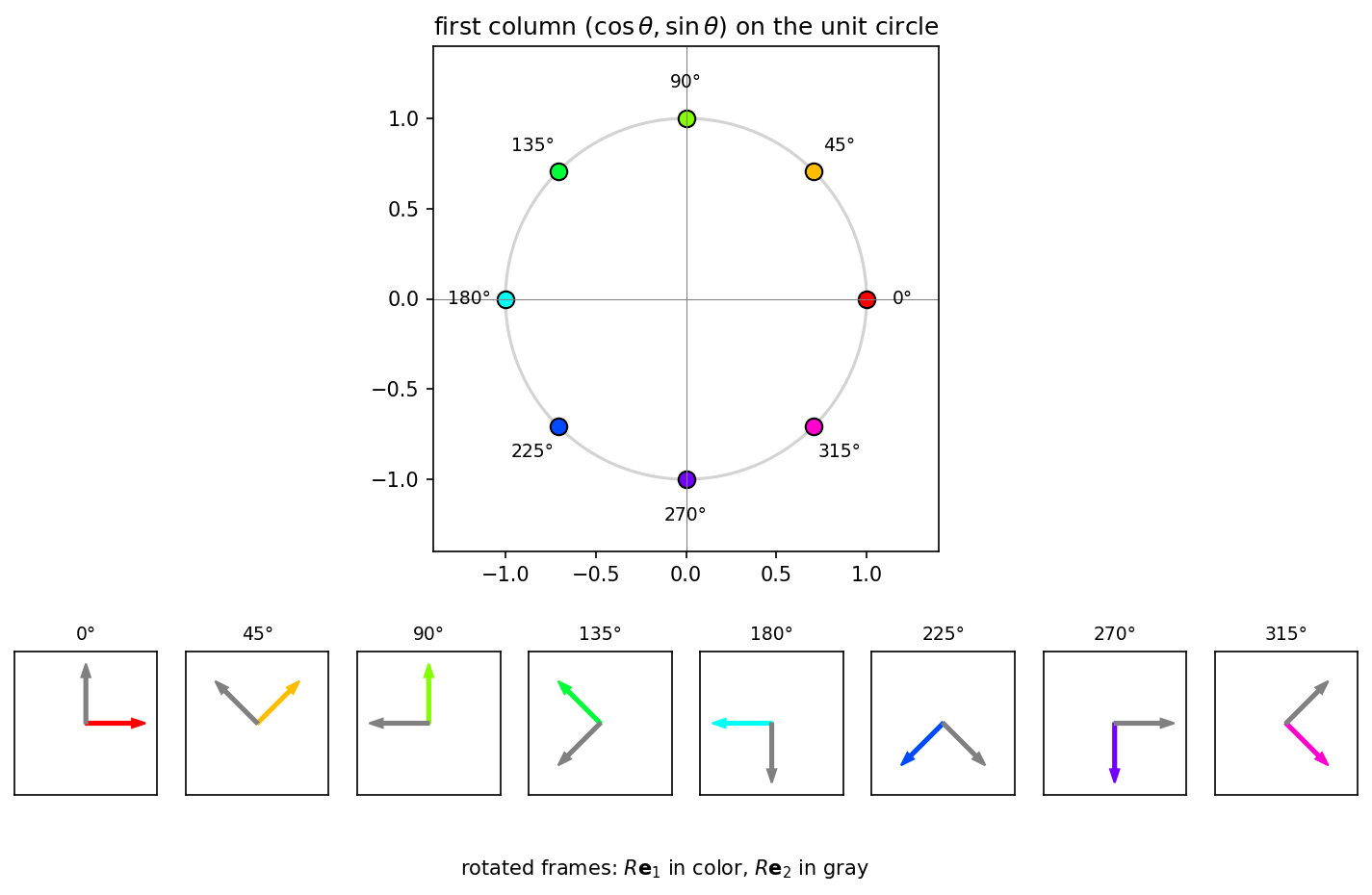
The first column of $R(\theta)$ is the image of the unit vector $\mathbf{e}_1$. It is the point $(\cos\theta, \sin\theta)$ on the unit circle in the plane. Once you know the first column, orthogonality and $\det R = +1$ determine the second. It is the first column turned by $90°$ counterclockwise. Every rotation therefore corresponds to exactly one point on the unit circle, and every point on the unit circle corresponds to exactly one rotation. This one-to-one correspondence identifies $SO(2)$ with a circle.
The top panel follows the first column as $\theta$ grows. The row below shows the full rotated frame $\{R\mathbf{e}_1, R\mathbf{e}_2\}$ at the same angles.
## One column is enough
The first column of $R(\theta)$ is the image of the unit vector $\mathbf{e}_1$. It is the point $(\cos\theta, \sin\theta)$ on the unit circle in the plane. Once you know the first column, orthogonality and $\det R = +1$ determine the second. It is the first column turned by $90°$ counterclockwise. Every rotation therefore corresponds to exactly one point on the unit circle, and every point on the unit circle corresponds to exactly one rotation. This one-to-one correspondence identifies $SO(2)$ with a circle.
The top panel follows the first column as $\theta$ grows. The row below shows the full rotated frame $\{R\mathbf{e}_1, R\mathbf{e}_2\}$ at the same angles.
 ## The tangent at the identity
A one-dimensional manifold looks like a straight line at sufficiently small scales. At the identity ($\theta = 0$), this line is tangent to the curve. Its direction is the derivative of $R(\theta)$ at $\theta = 0$:
$$
\left.\frac{dR}{d\theta}\right|_{\theta=0} = \begin{bmatrix} -\sin 0 & -\cos 0 \\ \cos 0 & -\sin 0 \end{bmatrix} = \begin{bmatrix} 0 & -1 \\ 1 & 0 \end{bmatrix}
$$
This skew-symmetric matrix is an element of $\mathfrak{so}(2)$. Call it $G$. Scaling it by an angular rate $\omega$ gives every possible velocity at the identity. Thus $\mathfrak{so}(2)$ is one-dimensional, like $SO(2)$.
The tangent space is a vector space. Each element is a linear combination of basis matrices called *generators*. For $SO(2)$ the tangent space is one-dimensional, so the single matrix $G$ is a basis:
$$
\mathfrak{so}(2) = \left\{ \omega G : \omega \in \mathbb{R} \right\} = \operatorname{span}\{G\}, \qquad G = \begin{bmatrix} 0 & -1 \\ 1 & 0 \end{bmatrix}
$$
The angular rate $\omega$ is the coordinate of a velocity in this basis. The matrix exponential maps back onto the curve: exponentiating $\theta G$ reproduces $R(\theta)$. Appendix D of Corke (Corke, 2023) develops the same construction step by step. It writes any $2 \times 2$ matrix as a combination of four basis matrices, places $SO(2)$ as a closed curve in that four-dimensional space, and repeats the construction for $SO(3)$, whose tangent space at the identity has three generators. [Lie groups and tangent spaces](/aiml-common/lectures/motion-algebras/lie-theory/index) presents the tangent space and exponential map in a broader setting. The calculation below checks the derivative, skew symmetry, and exponential map.
```python theme={null}
from scipy.linalg import expm
h = 1e-6
dR = (rot(h) - rot(-h)) / (2 * h) # central difference at theta = 0
print("dR/dtheta at identity:")
print(np.round(dR, 6))
print("skew-symmetric:", np.allclose(dR, -dR.T))
theta = 1.2
print(f"\nexp({theta} * dR) equals R({theta}):", np.allclose(expm(theta * dR), rot(theta)))
```
```output theme={null}
dR/dtheta at identity:
[[ 0. -1.]
[ 1. 0.]]
skew-symmetric: True
exp(1.2 * dR) equals R(1.2): True
```
## References
* Corke, P. (2023). *Robotics, vision and control: Fundamental algorithms in python*.
***
Found an error on this page? [Report an issue](https://github.com/aegean-ai/eaia-feedback/issues/new?template=page-issue.yml\&page=/aiml-common/lectures/motion-algebras/so2-manifold).
This documentation is built and hosted on [Mintlify](https://mintlify.com), a developer documentation platform.
## The tangent at the identity
A one-dimensional manifold looks like a straight line at sufficiently small scales. At the identity ($\theta = 0$), this line is tangent to the curve. Its direction is the derivative of $R(\theta)$ at $\theta = 0$:
$$
\left.\frac{dR}{d\theta}\right|_{\theta=0} = \begin{bmatrix} -\sin 0 & -\cos 0 \\ \cos 0 & -\sin 0 \end{bmatrix} = \begin{bmatrix} 0 & -1 \\ 1 & 0 \end{bmatrix}
$$
This skew-symmetric matrix is an element of $\mathfrak{so}(2)$. Call it $G$. Scaling it by an angular rate $\omega$ gives every possible velocity at the identity. Thus $\mathfrak{so}(2)$ is one-dimensional, like $SO(2)$.
The tangent space is a vector space. Each element is a linear combination of basis matrices called *generators*. For $SO(2)$ the tangent space is one-dimensional, so the single matrix $G$ is a basis:
$$
\mathfrak{so}(2) = \left\{ \omega G : \omega \in \mathbb{R} \right\} = \operatorname{span}\{G\}, \qquad G = \begin{bmatrix} 0 & -1 \\ 1 & 0 \end{bmatrix}
$$
The angular rate $\omega$ is the coordinate of a velocity in this basis. The matrix exponential maps back onto the curve: exponentiating $\theta G$ reproduces $R(\theta)$. Appendix D of Corke (Corke, 2023) develops the same construction step by step. It writes any $2 \times 2$ matrix as a combination of four basis matrices, places $SO(2)$ as a closed curve in that four-dimensional space, and repeats the construction for $SO(3)$, whose tangent space at the identity has three generators. [Lie groups and tangent spaces](/aiml-common/lectures/motion-algebras/lie-theory/index) presents the tangent space and exponential map in a broader setting. The calculation below checks the derivative, skew symmetry, and exponential map.
```python theme={null}
from scipy.linalg import expm
h = 1e-6
dR = (rot(h) - rot(-h)) / (2 * h) # central difference at theta = 0
print("dR/dtheta at identity:")
print(np.round(dR, 6))
print("skew-symmetric:", np.allclose(dR, -dR.T))
theta = 1.2
print(f"\nexp({theta} * dR) equals R({theta}):", np.allclose(expm(theta * dR), rot(theta)))
```
```output theme={null}
dR/dtheta at identity:
[[ 0. -1.]
[ 1. 0.]]
skew-symmetric: True
exp(1.2 * dR) equals R(1.2): True
```
## References
* Corke, P. (2023). *Robotics, vision and control: Fundamental algorithms in python*.
***
Found an error on this page? [Report an issue](https://github.com/aegean-ai/eaia-feedback/issues/new?template=page-issue.yml\&page=/aiml-common/lectures/motion-algebras/so2-manifold).
This documentation is built and hosted on [Mintlify](https://mintlify.com), a developer documentation platform.