> ## Documentation Index
> Fetch the complete documentation index at: https://aegean.ai/llms.txt
> Use this file to discover all available pages before exploring further.
# Scaled dot-product attention, a statistical perspective
> Why attention scores are divided by √d, variance analysis and demonstrations.
Consider query and key vectors $q, k \in \mathbb{R}^d$ with components assumed to be independent and identically distributed random variables:
$$
q_i, k_i \sim \mathcal{N}(0, \sigma^2)
$$
The dot product is:
$$
s = q \cdot k = \sum_{i=1}^d q_i k_i
$$
Since each term has mean zero and variance $\sigma^4$, we obtain:
$$
\mathrm{Var}(s) = d \sigma^4
$$
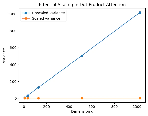
Thus, as the dimensionality $d$ increases, the variance of the dot product grows linearly, and its magnitude grows on the order of $\sqrt{d}$.
To stabilize this behavior, scaled dot-product attention introduces:
$$
\tilde{s} = \frac{q \cdot k}{\sqrt{d}}
$$
which yields:
$$
\mathrm{Var}(\tilde{s}) = \sigma^4
$$
This normalization ensures that the input to the softmax function remains well-conditioned, preventing saturation and preserving meaningful gradients during optimization.
This argument is consistent with principles from high-dimensional probability and statistical signal processing, where normalization by $\sqrt{d}$ preserves constant signal energy across dimensions.
```python theme={null}
# Demonstration: variance growth vs scaling
import numpy as np
import matplotlib.pyplot as plt
def simulate_variance(d, trials=10000):
q = np.random.randn(trials, d)
k = np.random.randn(trials, d)
dot = np.sum(q * k, axis=1)
scaled_dot = dot / np.sqrt(d)
return np.var(dot), np.var(scaled_dot)
dims = [8, 32, 128, 512, 1024]
var_raw = []
var_scaled = []
for d in dims:
v_raw, v_scaled = simulate_variance(d)
var_raw.append(v_raw)
var_scaled.append(v_scaled)
plt.figure()
plt.plot(dims, var_raw, marker='o', label='Unscaled variance')
plt.plot(dims, var_scaled, marker='o', label='Scaled variance')
plt.xlabel("Dimension d")
plt.ylabel("Variance")
plt.title("Effect of Scaling in Dot-Product Attention")
plt.legend()
plt.show()
```
 ## Understanding the division by √d
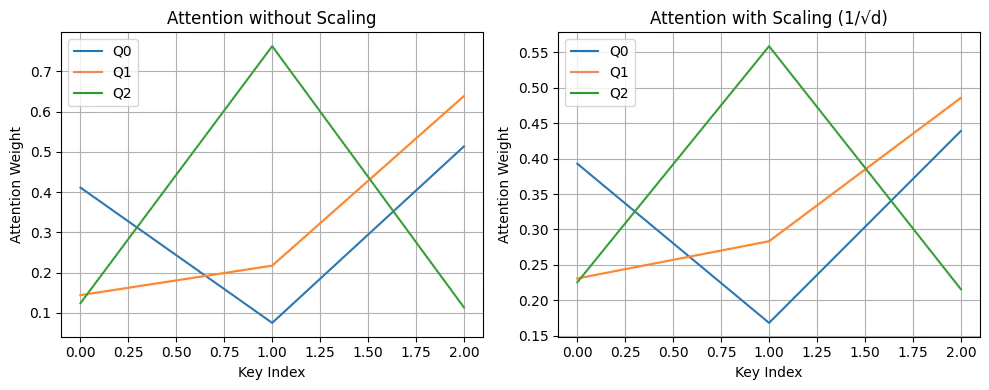
We use an example with embedding dimension $d = 4$, sequence length $T = 3$, and input vectors sampled from two Gaussian distributions.
* $Q, K \in \mathbb{R}^{T \times d}$
* Each row $q_i \sim \mathcal{N}(0, I_d)$, $k_j \sim \mathcal{N}(0, I_d)$
We compute:
$$
\text{score}_{ij} = q_i k_j^T = \sum_{\ell=1}^{d} q_{i\ell} k_{j\ell}
$$
Each component in the sum $q_{i\ell}k_{j\ell}$ is the product of two independent standard normal variables. The product of two independent standard normal variables follows a **standard normal product distribution**:
* Mean: $\mathbb{E}[XY] = 0$
* Variance: $\text{Var}[XY] = 1$
### Applying this to the dot product
Let:
$$
S = \sum_{\ell=1}^d q_{i\ell} k_{j\ell}
$$
Then:
* Each term has mean 0 and variance 1
* The terms are i.i.d. (since $Q$ and $K$ are independent)
* So: $\mathbb{E}[S] = 0$, $\text{Var}[S] = d$
The unscaled dot product therefore has **variance proportional to $d$**.
### Why divide by √d?
If we define the scaled score as:
$$
\text{scaled\_score}_{ij} = \frac{q_i \cdot k_j}{\sqrt{d}}
$$
Then:
$$
\text{Var}[\text{scaled\_score}_{ij}] = \frac{1}{d} \cdot \text{Var}[q_i \cdot k_j] = \frac{1}{d} \cdot d = 1
$$
The variance of the attention logits is **constant** regardless of dimension $d$, keeping the softmax numerically stable across different embedding sizes.
Without scaling, as $d$ grows the dot product variance grows linearly, causing the softmax to become extremely sharp, one large value dominates and others vanish, leading to poor gradient flow. With scaling, the dot product distribution is normalized and the softmax stays smooth and expressive.
```python theme={null}
import numpy as np
import matplotlib.pyplot as plt
# Settings
d = 4
T = 3
np.random.seed(42)
# Random Gaussian vectors for Q, K
Q = np.random.randn(T, d)
K = np.random.randn(T, d)
# Compute attention scores (dot product only)
dot_products = Q @ K.T
scaled_dot_products = dot_products / np.sqrt(d)
def softmax(x):
e_x = np.exp(x - np.max(x, axis=-1, keepdims=True))
return e_x / e_x.sum(axis=-1, keepdims=True)
# Compute softmax
attn_noscale = softmax(dot_products)
attn_scaled = softmax(scaled_dot_products)
attn_noscale, attn_scaled
```
```output theme={null}
(array([[0.41123254, 0.07536857, 0.51339889],
[0.14427532, 0.2173933 , 0.63833138],
[0.12411901, 0.76220571, 0.11367528]]),
array([[0.39285909, 0.16818537, 0.43895554],
[0.23089671, 0.28342933, 0.48567396],
[0.22547439, 0.55874566, 0.21577995]]))
```
```python theme={null}
fig, axs = plt.subplots(1, 2, figsize=(10, 4))
for i in range(T):
axs[0].plot(attn_noscale[i], label=f"Q{i}")
axs[1].plot(attn_scaled[i], label=f"Q{i}")
axs[0].set_title("Attention without Scaling")
axs[1].set_title("Attention with Scaling (1/√d)")
for ax in axs:
ax.set_xlabel("Key Index")
ax.set_ylabel("Attention Weight")
ax.legend()
ax.grid(True)
plt.tight_layout()
plt.show()
```
## Understanding the division by √d
We use an example with embedding dimension $d = 4$, sequence length $T = 3$, and input vectors sampled from two Gaussian distributions.
* $Q, K \in \mathbb{R}^{T \times d}$
* Each row $q_i \sim \mathcal{N}(0, I_d)$, $k_j \sim \mathcal{N}(0, I_d)$
We compute:
$$
\text{score}_{ij} = q_i k_j^T = \sum_{\ell=1}^{d} q_{i\ell} k_{j\ell}
$$
Each component in the sum $q_{i\ell}k_{j\ell}$ is the product of two independent standard normal variables. The product of two independent standard normal variables follows a **standard normal product distribution**:
* Mean: $\mathbb{E}[XY] = 0$
* Variance: $\text{Var}[XY] = 1$
### Applying this to the dot product
Let:
$$
S = \sum_{\ell=1}^d q_{i\ell} k_{j\ell}
$$
Then:
* Each term has mean 0 and variance 1
* The terms are i.i.d. (since $Q$ and $K$ are independent)
* So: $\mathbb{E}[S] = 0$, $\text{Var}[S] = d$
The unscaled dot product therefore has **variance proportional to $d$**.
### Why divide by √d?
If we define the scaled score as:
$$
\text{scaled\_score}_{ij} = \frac{q_i \cdot k_j}{\sqrt{d}}
$$
Then:
$$
\text{Var}[\text{scaled\_score}_{ij}] = \frac{1}{d} \cdot \text{Var}[q_i \cdot k_j] = \frac{1}{d} \cdot d = 1
$$
The variance of the attention logits is **constant** regardless of dimension $d$, keeping the softmax numerically stable across different embedding sizes.
Without scaling, as $d$ grows the dot product variance grows linearly, causing the softmax to become extremely sharp, one large value dominates and others vanish, leading to poor gradient flow. With scaling, the dot product distribution is normalized and the softmax stays smooth and expressive.
```python theme={null}
import numpy as np
import matplotlib.pyplot as plt
# Settings
d = 4
T = 3
np.random.seed(42)
# Random Gaussian vectors for Q, K
Q = np.random.randn(T, d)
K = np.random.randn(T, d)
# Compute attention scores (dot product only)
dot_products = Q @ K.T
scaled_dot_products = dot_products / np.sqrt(d)
def softmax(x):
e_x = np.exp(x - np.max(x, axis=-1, keepdims=True))
return e_x / e_x.sum(axis=-1, keepdims=True)
# Compute softmax
attn_noscale = softmax(dot_products)
attn_scaled = softmax(scaled_dot_products)
attn_noscale, attn_scaled
```
```output theme={null}
(array([[0.41123254, 0.07536857, 0.51339889],
[0.14427532, 0.2173933 , 0.63833138],
[0.12411901, 0.76220571, 0.11367528]]),
array([[0.39285909, 0.16818537, 0.43895554],
[0.23089671, 0.28342933, 0.48567396],
[0.22547439, 0.55874566, 0.21577995]]))
```
```python theme={null}
fig, axs = plt.subplots(1, 2, figsize=(10, 4))
for i in range(T):
axs[0].plot(attn_noscale[i], label=f"Q{i}")
axs[1].plot(attn_scaled[i], label=f"Q{i}")
axs[0].set_title("Attention without Scaling")
axs[1].set_title("Attention with Scaling (1/√d)")
for ax in axs:
ax.set_xlabel("Key Index")
ax.set_ylabel("Attention Weight")
ax.legend()
ax.grid(True)
plt.tight_layout()
plt.show()
```
 ## Summary
* Without scaling, attention scores can be overly large, leading to softmax outputs that are near one-hot.
* This results in vanishing gradients and unstable training.
* Scaling by $\frac{1}{\sqrt{d}}$ normalizes the variance of the dot product, improving gradient flow and model stability.
## PyTorch reference
| PyTorch class | Description |
| -------------------------------------------------------------------------------------------------------- | ------------------------------------------------------------------------------------------ |
| [`nn.Linear`](https://docs.pytorch.org/docs/2.12/generated/torch.nn.Linear.html) | Applies an affine linear transformation to the incoming data: $y = xA^T + b$. |
| [`nn.Softmax`](https://docs.pytorch.org/docs/2.12/generated/torch.nn.Softmax.html) | Applies the Softmax function to an n-dimensional input Tensor. |
| [`nn.MultiheadAttention`](https://docs.pytorch.org/docs/2.12/generated/torch.nn.MultiheadAttention.html) | Allows the model to jointly attend to information from different representation subspaces. |
***
[Edit this page on GitHub](https://github.com/aegean-ai/eaia/edit/main/src/aiml-common/lectures/nlp/transformers/attention-scaling-explained/attention_scaling_explained.mdx) or [file an issue](https://github.com/aegean-ai/eaia/issues/new/choose).
## Summary
* Without scaling, attention scores can be overly large, leading to softmax outputs that are near one-hot.
* This results in vanishing gradients and unstable training.
* Scaling by $\frac{1}{\sqrt{d}}$ normalizes the variance of the dot product, improving gradient flow and model stability.
## PyTorch reference
| PyTorch class | Description |
| -------------------------------------------------------------------------------------------------------- | ------------------------------------------------------------------------------------------ |
| [`nn.Linear`](https://docs.pytorch.org/docs/2.12/generated/torch.nn.Linear.html) | Applies an affine linear transformation to the incoming data: $y = xA^T + b$. |
| [`nn.Softmax`](https://docs.pytorch.org/docs/2.12/generated/torch.nn.Softmax.html) | Applies the Softmax function to an n-dimensional input Tensor. |
| [`nn.MultiheadAttention`](https://docs.pytorch.org/docs/2.12/generated/torch.nn.MultiheadAttention.html) | Allows the model to jointly attend to information from different representation subspaces. |
***
[Edit this page on GitHub](https://github.com/aegean-ai/eaia/edit/main/src/aiml-common/lectures/nlp/transformers/attention-scaling-explained/attention_scaling_explained.mdx) or [file an issue](https://github.com/aegean-ai/eaia/issues/new/choose).