> ## Documentation Index
> Fetch the complete documentation index at: https://aegean.ai/llms.txt
> Use this file to discover all available pages before exploring further.
# Maximum Likelihood Estimation of a Marginal Model
> Introduction to the Maximum Likelihood principle for estimating probability distributions from data.
Most of the models in supervised machine learning are estimated using the ML principle. In this section we introduce the principle and outline the objective function of the ML estimator that has wide applicability in many learning tasks. Assume that we have $m$ examples drawn from a data generator that generates the vectors $\mathbf{x} \in \mathcal{X}$ *independently and identically distributed (i.i.d.)* according to some unknown (but fixed) probability distribution function $p_{data}(\mathbf{x})$.
$\mathbb{X} = \{ \mathbf{x}_1, \dots, \mathbf{x}_m \}$
Let $p_{model}(\mathbf x, \mathbf w)$ a parametric family of probability distributions (our hypothesis set) over the same space that attempts to approximate (model) $p_{data}(\mathbf{x})$ as closely as possible using a suitable estimate of the parameter vector $\mathbf w$. The ML estimator for $\mathbf w$ is defined as:
$\mathbf w_{ML} = \underset{\mathbf w}{\text{argmax}} \, p_{model}(\mathbb X; \mathbf w)$
$= \underset{\mathbf w}{\text{argmax}} \prod_{i=1}^m p_{model}(\mathbf x^{(i)}; \mathbf w)$
$= \underset{\mathbf w}{\text{argmax}} \sum_{i=1}^m \log p_{model}(\mathbf x^{(i)}; \mathbf w)$
$= \underset{\mathbf w}{\text{argmax}} \frac{1}{m} \sum_{i=1}^m \log p_{model}(\mathbf x^{(i)}; \mathbf w)$
$= \underset{\mathbf w}{\text{argmax}} \, \mathbb{E}_{\mathbf{x} \sim \hat p_{data}} \log p_{model}(\mathbf x; \mathbf w)$
From the last expression it is evident that in ML estimation two distributions are involved: $\hat p_{data}$ and $p_{model}$. We can also make use of our intuition that a good estimator would minimize the distance between the two empirical distributions therefore the KL divergence:
$KL( \hat p_{data} \| p_{model} ) = \mathbb{E}_{\mathbf x \sim \hat p_{data}} \left[\log \hat p_{data}(\mathbf x) - \log p_{model}(\mathbf x, \mathbf w) \right]$
The first term is independent of the model and therefore we see that the KL and the ML estimator expressions are *identical* except from the sign. Therefore we conclude that *minimizing KL divergence, maximizes the likelihood function*. From information theory we know that the KL divergence and the cross entropy (CE) are related via the expression
$CE = H(\hat p_{data}, p_{model}) = KL( \hat p_{data} \| p_{model} ) + H(\hat p_{data})$
Given that $\hat p_{data}$ is given in supervised learning, $H(\hat p_{data})$ is constant and therefore we can conclude that in this case, CE is equivalent to the KL i.e. **minimizing the KL divergence, is equivalent in minimizing cross-entropy (CE)**. Therefore the expression the only need to minimize which we will call the CE cost function (also known as log loss) is:
$L(\mathbf w) = CE = - \mathbb{E}_{\mathbf x \sim \hat p_{data}} \log p_{model}(\mathbf x, \mathbf w)$
Cross entropy is a very generic objective (loss) function that is applicable to any *supervised learning* problem that uses maximum likelihood to estimate a model.
## Visualizing MLE with a Gaussian
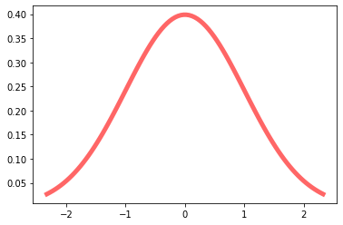
To visualize the above, let's start with a simple Gaussian distribution.
```python theme={null}
import numpy as np
from scipy.stats import norm
import matplotlib.pyplot as plt
fig, ax = plt.subplots(1, 1)
x = np.linspace(norm.ppf(0.01), norm.ppf(0.99), 100)
ax.plot(x, norm.pdf(x), 'r-', lw=5, alpha=0.6, label='norm pdf')
```
 We can retrieve the probability of events happening, e.g. x=3.0:
```python theme={null}
p_3 = norm.pdf(3.0, 5.0, 3.0)
```
We can also easily calculate the joint probability of i.i.d. (independent and identically distributed) events:
```python theme={null}
p_7 = norm.pdf(7.0, 7.0, 3.0)
joint = p_3 * p_7
```
## Comparing Hypotheses
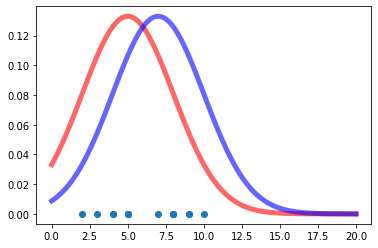
Assume now that someone is giving us an array of values and ask us to estimate a $p_{model}$ that is a 'good fit' to the given data. How can we go about solving this problem with Maximum Likelihood Estimation (MLE)?
Notice that probability and likelihood have a reverse relationship. Probability attaches to possible results; likelihood attaches to hypotheses. The likelihood function gives the relative likelihoods of different values for the parameter(s) of the distribution from which the data are assumed to have been drawn, given those data.
```python theme={null}
data = [4, 5, 7, 8, 8, 9, 10, 5, 2, 3, 5, 4, 8, 9]
fig, ax = plt.subplots(1, 1)
x = np.linspace(0, 20, 100)
ax.plot(x, norm.pdf(x, 5, 3), 'r-', lw=5, alpha=0.6, label='μ=5')
ax.plot(x, norm.pdf(x, 7, 3), 'b-', lw=5, alpha=0.6, label='μ=7')
ax.plot(data, np.zeros(len(data)).tolist(), 'o')
```
We can retrieve the probability of events happening, e.g. x=3.0:
```python theme={null}
p_3 = norm.pdf(3.0, 5.0, 3.0)
```
We can also easily calculate the joint probability of i.i.d. (independent and identically distributed) events:
```python theme={null}
p_7 = norm.pdf(7.0, 7.0, 3.0)
joint = p_3 * p_7
```
## Comparing Hypotheses
Assume now that someone is giving us an array of values and ask us to estimate a $p_{model}$ that is a 'good fit' to the given data. How can we go about solving this problem with Maximum Likelihood Estimation (MLE)?
Notice that probability and likelihood have a reverse relationship. Probability attaches to possible results; likelihood attaches to hypotheses. The likelihood function gives the relative likelihoods of different values for the parameter(s) of the distribution from which the data are assumed to have been drawn, given those data.
```python theme={null}
data = [4, 5, 7, 8, 8, 9, 10, 5, 2, 3, 5, 4, 8, 9]
fig, ax = plt.subplots(1, 1)
x = np.linspace(0, 20, 100)
ax.plot(x, norm.pdf(x, 5, 3), 'r-', lw=5, alpha=0.6, label='μ=5')
ax.plot(x, norm.pdf(x, 7, 3), 'b-', lw=5, alpha=0.6, label='μ=7')
ax.plot(data, np.zeros(len(data)).tolist(), 'o')
```
 ## Computing Log-Likelihood
It's important to safeguard against underflow that may result from multiplying many numbers (for large datasets) that are less than 1.0 (probabilities). So we do the calculations in the log domain using the identity:
$\log(a \times b) = \log(a) + \log(b)$
Let's look at a function that calculates the log-likelihood for two hypotheses given the data:
```python theme={null}
def compare_data_to_dist(x, mu_1=5, mu_2=7, sd_1=3, sd_2=3):
ll_1 = 0
ll_2 = 0
for i in x:
ll_1 += np.log(norm.pdf(i, mu_1, sd_1))
ll_2 += np.log(norm.pdf(i, mu_2, sd_2))
print(f"The LL for μ={mu_1}, σ={sd_1} is: {ll_1:.4f}")
print(f"The LL for μ={mu_2}, σ={sd_2} is: {ll_2:.4f}")
```
We can readily compare the two hypotheses according to the maximum likelihood criterion. Note that because the $\log$ is a monotonic function, the conclusion as to which hypothesis makes the data more likely is the same in the natural or the $\log$ domain.
```python theme={null}
ll_comparison = compare_data_to_dist(data)
# Output:
# The LL for μ=5, σ=3 is: -33.9679
# The LL for μ=7, σ=3 is: -33.3013
```
It seems that the second hypothesis $p_{model}(x \mid \mathbf{w}) = \mathcal{N}(x \mid \mu_2, \sigma_2^2)$ is preferred compared to the first.
## Searching the Parameter Space
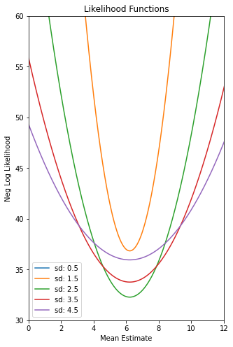
We can search the hypothesis space (parameter space) for the best parameter set $\mathbf w$:
```python theme={null}
def plot_ll(x):
plt.figure(figsize=(5, 8))
plt.title("Negative Log Likelihood Functions")
plt.xlabel("Mean Estimate")
plt.ylabel("Negative Log Likelihood")
mu_set = np.linspace(0, 16, 1000)
sd_set = [0.5, 1.5, 2.5, 3.5, 4.5]
for sd in sd_set:
ll_array = []
for mu in mu_set:
temp_ll = sum(np.log(norm.pdf(k, mu, sd)) for k in x)
ll_array.append(-temp_ll) # negative LL
plt.plot(mu_set, ll_array, label=f"σ={sd}")
plt.legend(loc='lower left')
plt.show()
plot_ll(data)
```
## Computing Log-Likelihood
It's important to safeguard against underflow that may result from multiplying many numbers (for large datasets) that are less than 1.0 (probabilities). So we do the calculations in the log domain using the identity:
$\log(a \times b) = \log(a) + \log(b)$
Let's look at a function that calculates the log-likelihood for two hypotheses given the data:
```python theme={null}
def compare_data_to_dist(x, mu_1=5, mu_2=7, sd_1=3, sd_2=3):
ll_1 = 0
ll_2 = 0
for i in x:
ll_1 += np.log(norm.pdf(i, mu_1, sd_1))
ll_2 += np.log(norm.pdf(i, mu_2, sd_2))
print(f"The LL for μ={mu_1}, σ={sd_1} is: {ll_1:.4f}")
print(f"The LL for μ={mu_2}, σ={sd_2} is: {ll_2:.4f}")
```
We can readily compare the two hypotheses according to the maximum likelihood criterion. Note that because the $\log$ is a monotonic function, the conclusion as to which hypothesis makes the data more likely is the same in the natural or the $\log$ domain.
```python theme={null}
ll_comparison = compare_data_to_dist(data)
# Output:
# The LL for μ=5, σ=3 is: -33.9679
# The LL for μ=7, σ=3 is: -33.3013
```
It seems that the second hypothesis $p_{model}(x \mid \mathbf{w}) = \mathcal{N}(x \mid \mu_2, \sigma_2^2)$ is preferred compared to the first.
## Searching the Parameter Space
We can search the hypothesis space (parameter space) for the best parameter set $\mathbf w$:
```python theme={null}
def plot_ll(x):
plt.figure(figsize=(5, 8))
plt.title("Negative Log Likelihood Functions")
plt.xlabel("Mean Estimate")
plt.ylabel("Negative Log Likelihood")
mu_set = np.linspace(0, 16, 1000)
sd_set = [0.5, 1.5, 2.5, 3.5, 4.5]
for sd in sd_set:
ll_array = []
for mu in mu_set:
temp_ll = sum(np.log(norm.pdf(k, mu, sd)) for k in x)
ll_array.append(-temp_ll) # negative LL
plt.plot(mu_set, ll_array, label=f"σ={sd}")
plt.legend(loc='lower left')
plt.show()
plot_ll(data)
```
 But there is a better method than exhaustively searching in the parameter space. We developed a method that incrementally minimizes a loss function that is ultimately linked to the concept of entropy - the cross entropy (CE) that for the supervised learning problem as shown in the notes has a lot to do with minimizing the KL divergence - a type of probabilistic 'distance' between $\hat p_{data}$ and $p_{model}$.
This method is the **Stochastic Gradient Descent** as described in the [SGD lecture](/aiml-common/lectures/optimization/sgd/index).
## References
1. [Maximum Likelihood Estimation of Gaussian Parameters](/aiml-common/lectures/optimization/maximum-likelihood/mle-gaussian-parameters) - Detailed derivation of MLE for Gaussian parameters
2. [Section 4.1 - Numerical computation](https://www.deeplearningbook.org/contents/numerical.html) - Deep Learning Book
3. [Bayes for beginners - probability and likelihood](https://www.psychologicalscience.org/observer/bayes-for-beginners-probability-and-likelihood)
***
[Edit this page on GitHub](https://github.com/aegean-ai/eaia/edit/main/src/aiml-common/lectures/optimization/maximum-likelihood/marginal_maximum_likelihood.mdx) or [file an issue](https://github.com/aegean-ai/eaia/issues/new/choose).
But there is a better method than exhaustively searching in the parameter space. We developed a method that incrementally minimizes a loss function that is ultimately linked to the concept of entropy - the cross entropy (CE) that for the supervised learning problem as shown in the notes has a lot to do with minimizing the KL divergence - a type of probabilistic 'distance' between $\hat p_{data}$ and $p_{model}$.
This method is the **Stochastic Gradient Descent** as described in the [SGD lecture](/aiml-common/lectures/optimization/sgd/index).
## References
1. [Maximum Likelihood Estimation of Gaussian Parameters](/aiml-common/lectures/optimization/maximum-likelihood/mle-gaussian-parameters) - Detailed derivation of MLE for Gaussian parameters
2. [Section 4.1 - Numerical computation](https://www.deeplearningbook.org/contents/numerical.html) - Deep Learning Book
3. [Bayes for beginners - probability and likelihood](https://www.psychologicalscience.org/observer/bayes-for-beginners-probability-and-likelihood)
***
[Edit this page on GitHub](https://github.com/aegean-ai/eaia/edit/main/src/aiml-common/lectures/optimization/maximum-likelihood/marginal_maximum_likelihood.mdx) or [file an issue](https://github.com/aegean-ai/eaia/issues/new/choose).