> ## Documentation Index
> Fetch the complete documentation index at: https://aegean.ai/llms.txt
> Use this file to discover all available pages before exploring further.
# Optimization Algorithms
> Gradient descent, stochastic and mini-batch SGD, and learning-rate schedules, built from scratch in NumPy with a PyTorch coda.
 Training a model means searching the weight space for the parameters that minimize a loss. This section builds that search from the ground up: plain **gradient descent** on a convex objective, then the **stochastic** and **mini-batch** variants that let it scale to large datasets, and finally the same loop expressed with PyTorch. It is the engine behind the [linear regression](/aiml-common/lectures/regression/linear-regression) fits and, eventually, deep-network training. The loss being minimized is the empirical risk defined on the [empirical and expected risk](/aiml-common/lectures/empirical-risk) page.
## Gradient descent
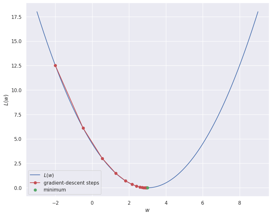
Optimization minimizes a function $L(\boldsymbol{\theta})$ by adjusting $\boldsymbol{\theta}$. The derivative $L'(w)$ gives the slope: to first order $L(w + \epsilon) \approx L(w) + \epsilon\, L'(w)$, so moving a small step *against* the derivative decreases $L$. For a vector of weights the gradient $\nabla_{\boldsymbol{\theta}} L$ collects all partial derivatives, and gradient descent repeatedly steps downhill,
$\boldsymbol{\theta}_{k+1} = \boldsymbol{\theta}_k - \eta\, \nabla_{\boldsymbol{\theta}} L(\boldsymbol{\theta}_k),$
where the **learning rate** $\eta$ scales the step. On a convex bowl the iterates march steadily to the unique minimum.
```python theme={null}
def L(w):
return 0.5 * (w - 3.0) ** 2 # convex bowl, minimum at w = 3
def dL(w):
return w - 3.0
w, eta, traj = -2.0, 0.3, [-2.0]
for _ in range(15):
w = w - eta * dL(w)
traj.append(w)
traj = np.array(traj)
print(f"start w = {traj[0]:.2f} -> final w = {traj[-1]:.4f} (true minimum at w = 3)")
```
```output theme={null}
start w = -2.00 -> final w = 2.9763 (true minimum at w = 3)
```
Training a model means searching the weight space for the parameters that minimize a loss. This section builds that search from the ground up: plain **gradient descent** on a convex objective, then the **stochastic** and **mini-batch** variants that let it scale to large datasets, and finally the same loop expressed with PyTorch. It is the engine behind the [linear regression](/aiml-common/lectures/regression/linear-regression) fits and, eventually, deep-network training. The loss being minimized is the empirical risk defined on the [empirical and expected risk](/aiml-common/lectures/empirical-risk) page.
## Gradient descent
Optimization minimizes a function $L(\boldsymbol{\theta})$ by adjusting $\boldsymbol{\theta}$. The derivative $L'(w)$ gives the slope: to first order $L(w + \epsilon) \approx L(w) + \epsilon\, L'(w)$, so moving a small step *against* the derivative decreases $L$. For a vector of weights the gradient $\nabla_{\boldsymbol{\theta}} L$ collects all partial derivatives, and gradient descent repeatedly steps downhill,
$\boldsymbol{\theta}_{k+1} = \boldsymbol{\theta}_k - \eta\, \nabla_{\boldsymbol{\theta}} L(\boldsymbol{\theta}_k),$
where the **learning rate** $\eta$ scales the step. On a convex bowl the iterates march steadily to the unique minimum.
```python theme={null}
def L(w):
return 0.5 * (w - 3.0) ** 2 # convex bowl, minimum at w = 3
def dL(w):
return w - 3.0
w, eta, traj = -2.0, 0.3, [-2.0]
for _ in range(15):
w = w - eta * dL(w)
traj.append(w)
traj = np.array(traj)
print(f"start w = {traj[0]:.2f} -> final w = {traj[-1]:.4f} (true minimum at w = 3)")
```
```output theme={null}
start w = -2.00 -> final w = 2.9763 (true minimum at w = 3)
```
 ## The learning rate
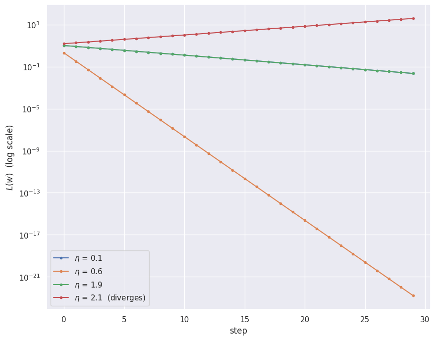
The learning rate sets the size of each step and is the most important knob. Too small and progress is glacial; too large and the steps overshoot the minimum and the iterates oscillate or diverge. For the quadratic above the update contracts the distance to the minimum by a factor $|1 - \eta|$ per step, so anything with $\eta > 2$ blows up.
```python theme={null}
def run_gd(eta, steps=30, w0=-2.0):
w, hist = w0, []
for _ in range(steps):
w = w - eta * dL(w)
hist.append(L(w))
return np.array(hist)
etas = [0.1, 0.6, 1.9, 2.1]
curves = {eta: run_gd(eta) for eta in etas}
```
## The learning rate
The learning rate sets the size of each step and is the most important knob. Too small and progress is glacial; too large and the steps overshoot the minimum and the iterates oscillate or diverge. For the quadratic above the update contracts the distance to the minimum by a factor $|1 - \eta|$ per step, so anything with $\eta > 2$ blows up.
```python theme={null}
def run_gd(eta, steps=30, w0=-2.0):
w, hist = w0, []
for _ in range(steps):
w = w - eta * dL(w)
hist.append(L(w))
return np.array(hist)
etas = [0.1, 0.6, 1.9, 2.1]
curves = {eta: run_gd(eta) for eta in etas}
```
 ## From full-batch to stochastic
In learning the loss is an **average over the training set**, and so is its gradient. For squared error with $m$ examples,
$L(\boldsymbol{\theta}) = \frac{1}{m}\sum_{i=1}^{m}\big(\boldsymbol{\theta}^{\top}\mathbf{x}_i - y_i\big)^2, \qquad \nabla_{\boldsymbol{\theta}} L = \frac{2}{m}\sum_{i=1}^{m}\big(\boldsymbol{\theta}^{\top}\mathbf{x}_i - y_i\big)\mathbf{x}_i.$
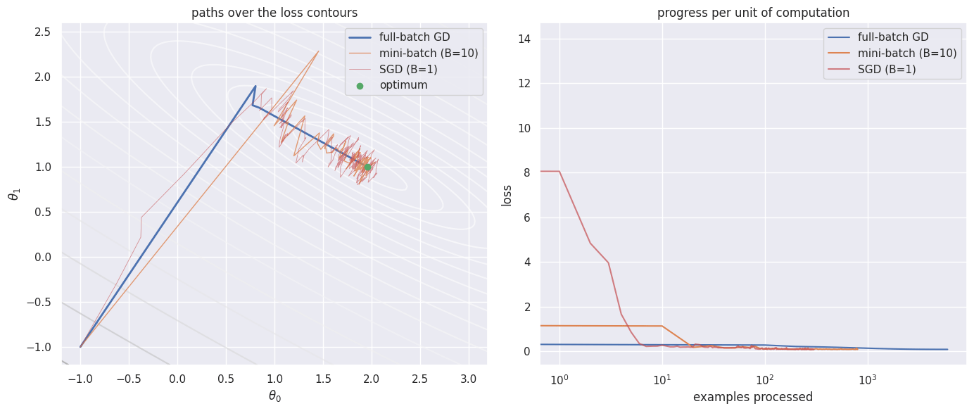
**Full-batch** gradient descent sums over all $m$ examples for every single update. With millions of examples that is prohibitive. Instead you estimate the gradient on a random **mini-batch** $\mathcal{B}$ of size $B$; the special case $B = 1$ is **stochastic gradient descent**. The mini-batch gradient is an unbiased but noisy estimate of the full gradient, so each step is cheap and frequent, at the cost of a wandering trajectory.
To see all three on one picture, fit a straight line $y = \theta_0 x + \theta_1$ to noisy data: the loss over the two parameters is a bowl whose contours you can draw.
```python theme={null}
m = 100
x = rng.uniform(0, 1, m)
y = 2.0 * x + 1.0 + rng.normal(0, 0.3, m) # true line theta = [2, 1] plus noise
X = np.c_[x, np.ones(m)] # design columns [x, 1]
def loss(theta):
return np.mean((X @ theta - y) ** 2)
def grad(theta, idx):
Xb, yb = X[idx], y[idx]
return (2 / len(idx)) * (Xb.T @ (Xb @ theta - yb))
theta_star = np.linalg.solve(X.T @ X, X.T @ y) # least-squares optimum
def descend(batch_size, epochs, eta, seed=0):
g = np.random.default_rng(seed)
theta = np.array([-1.0, -1.0])
path, seen, cost = [theta.copy()], [0], 0
losses = [loss(theta)]
for _ in range(epochs):
order = g.permutation(m)
for s in range(0, m, batch_size):
idx = order[s:s + batch_size]
theta = theta - eta * grad(theta, idx)
cost += len(idx)
path.append(theta.copy()); seen.append(cost); losses.append(loss(theta))
return np.array(path), np.array(seen), np.array(losses)
gd_path, gd_seen, gd_loss = descend(batch_size=m, epochs=60, eta=0.4) # full batch
mb_path, mb_seen, mb_loss = descend(batch_size=10, epochs=8, eta=0.4) # mini-batch
sgd_path, sgd_seen, sgd_loss = descend(batch_size=1, epochs=3, eta=0.1) # SGD
print("optimum theta* =", np.round(theta_star, 3))
```
```output theme={null}
optimum theta* = [1.961 0.998]
```
## From full-batch to stochastic
In learning the loss is an **average over the training set**, and so is its gradient. For squared error with $m$ examples,
$L(\boldsymbol{\theta}) = \frac{1}{m}\sum_{i=1}^{m}\big(\boldsymbol{\theta}^{\top}\mathbf{x}_i - y_i\big)^2, \qquad \nabla_{\boldsymbol{\theta}} L = \frac{2}{m}\sum_{i=1}^{m}\big(\boldsymbol{\theta}^{\top}\mathbf{x}_i - y_i\big)\mathbf{x}_i.$
**Full-batch** gradient descent sums over all $m$ examples for every single update. With millions of examples that is prohibitive. Instead you estimate the gradient on a random **mini-batch** $\mathcal{B}$ of size $B$; the special case $B = 1$ is **stochastic gradient descent**. The mini-batch gradient is an unbiased but noisy estimate of the full gradient, so each step is cheap and frequent, at the cost of a wandering trajectory.
To see all three on one picture, fit a straight line $y = \theta_0 x + \theta_1$ to noisy data: the loss over the two parameters is a bowl whose contours you can draw.
```python theme={null}
m = 100
x = rng.uniform(0, 1, m)
y = 2.0 * x + 1.0 + rng.normal(0, 0.3, m) # true line theta = [2, 1] plus noise
X = np.c_[x, np.ones(m)] # design columns [x, 1]
def loss(theta):
return np.mean((X @ theta - y) ** 2)
def grad(theta, idx):
Xb, yb = X[idx], y[idx]
return (2 / len(idx)) * (Xb.T @ (Xb @ theta - yb))
theta_star = np.linalg.solve(X.T @ X, X.T @ y) # least-squares optimum
def descend(batch_size, epochs, eta, seed=0):
g = np.random.default_rng(seed)
theta = np.array([-1.0, -1.0])
path, seen, cost = [theta.copy()], [0], 0
losses = [loss(theta)]
for _ in range(epochs):
order = g.permutation(m)
for s in range(0, m, batch_size):
idx = order[s:s + batch_size]
theta = theta - eta * grad(theta, idx)
cost += len(idx)
path.append(theta.copy()); seen.append(cost); losses.append(loss(theta))
return np.array(path), np.array(seen), np.array(losses)
gd_path, gd_seen, gd_loss = descend(batch_size=m, epochs=60, eta=0.4) # full batch
mb_path, mb_seen, mb_loss = descend(batch_size=10, epochs=8, eta=0.4) # mini-batch
sgd_path, sgd_seen, sgd_loss = descend(batch_size=1, epochs=3, eta=0.1) # SGD
print("optimum theta* =", np.round(theta_star, 3))
```
```output theme={null}
optimum theta* = [1.961 0.998]
```
 ## Gradient noise and learning-rate schedules
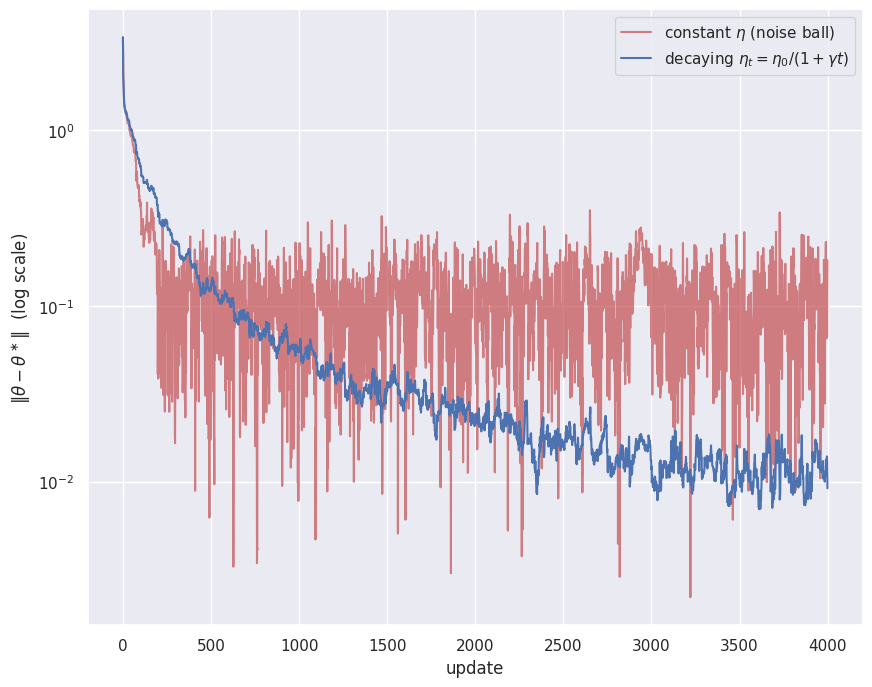
With a *constant* learning rate the stochastic gradient never vanishes, even at the optimum a single mini-batch still pulls in some direction. The iterate therefore settles into a **noise ball** around the minimum whose radius scales with $\eta$, bouncing rather than converging. Shrinking the learning rate over time, for example $\eta_t = \eta_0 / (1 + \gamma t)$, lets the ball contract so the iterate homes in. This is exactly the gap between the constant-rate and converged fits seen on the regression [SGD example](/aiml-common/lectures/regression/linear-regression/sgd/sgd_sinusoidal_dataset).
```python theme={null}
def sgd_schedule(eta0, decay, epochs=40, seed=1):
g = np.random.default_rng(seed)
theta, dist, t = np.array([-1.0, -1.0]), [], 0
for _ in range(epochs):
for i in g.permutation(m):
eta = eta0 / (1 + decay * t)
theta = theta - eta * grad(theta, [i])
dist.append(np.linalg.norm(theta - theta_star)); t += 1
return np.array(dist)
dist_const = sgd_schedule(0.1, 0.0) # constant learning rate
dist_decay = sgd_schedule(0.1, 0.01) # decaying learning rate
print(f"constant-eta final distance to optimum : {dist_const[-1]:.3f}")
print(f"decaying-eta final distance to optimum : {dist_decay[-1]:.3f}")
```
```output theme={null}
constant-eta final distance to optimum : 0.182
decaying-eta final distance to optimum : 0.009
```
## Gradient noise and learning-rate schedules
With a *constant* learning rate the stochastic gradient never vanishes, even at the optimum a single mini-batch still pulls in some direction. The iterate therefore settles into a **noise ball** around the minimum whose radius scales with $\eta$, bouncing rather than converging. Shrinking the learning rate over time, for example $\eta_t = \eta_0 / (1 + \gamma t)$, lets the ball contract so the iterate homes in. This is exactly the gap between the constant-rate and converged fits seen on the regression [SGD example](/aiml-common/lectures/regression/linear-regression/sgd/sgd_sinusoidal_dataset).
```python theme={null}
def sgd_schedule(eta0, decay, epochs=40, seed=1):
g = np.random.default_rng(seed)
theta, dist, t = np.array([-1.0, -1.0]), [], 0
for _ in range(epochs):
for i in g.permutation(m):
eta = eta0 / (1 + decay * t)
theta = theta - eta * grad(theta, [i])
dist.append(np.linalg.norm(theta - theta_star)); t += 1
return np.array(dist)
dist_const = sgd_schedule(0.1, 0.0) # constant learning rate
dist_decay = sgd_schedule(0.1, 0.01) # decaying learning rate
print(f"constant-eta final distance to optimum : {dist_const[-1]:.3f}")
print(f"decaying-eta final distance to optimum : {dist_decay[-1]:.3f}")
```
```output theme={null}
constant-eta final distance to optimum : 0.182
decaying-eta final distance to optimum : 0.009
```
 ## The same loop in PyTorch
Frameworks automate two things you did by hand: autograd computes $\nabla_{\boldsymbol{\theta}} L$ from the forward computation, and an optimizer object applies the update rule. The mechanics are identical, `loss.backward()` fills in the gradient and `optimizer.step()` performs $\boldsymbol{\theta} \leftarrow \boldsymbol{\theta} - \eta\nabla_{\boldsymbol{\theta}} L$.
```python theme={null}
import torch
Xt = torch.tensor(X, dtype=torch.float32)
yt = torch.tensor(y, dtype=torch.float32)
theta = torch.tensor([-1.0, -1.0], requires_grad=True)
optimizer = torch.optim.SGD([theta], lr=0.4)
for epoch in range(200):
optimizer.zero_grad()
loss_t = ((Xt @ theta - yt) ** 2).mean()
loss_t.backward() # autograd fills theta.grad
optimizer.step() # theta <- theta - lr * theta.grad
print("PyTorch SGD theta =", np.round(theta.detach().numpy(), 3))
print("least squares theta* =", np.round(theta_star, 3))
```
```output theme={null}
PyTorch SGD theta = [1.961 0.998]
least squares theta* = [1.961 0.998]
```
## Takeaways
* Gradient descent steps against the gradient; the learning rate $\eta$ sets the step size, and too large a value diverges.
* The training loss is an average over data, so its gradient is too. Full-batch updates cost a complete pass, while mini-batch and stochastic updates trade gradient noise for cheap, frequent steps that make far more progress per unit of computation.
* A constant learning rate leaves stochastic gradient descent circling in a noise ball; a decaying schedule lets it converge.
* Autograd plus an optimizer object package this exact loop. The [optimizer zoo](/aiml-common/lectures/optimization/optimizers) section adds momentum and adaptive methods that handle the ill-conditioned, ravine-shaped landscapes where plain SGD struggles.
**Key references**: (Bottou et al., 2016; Goodfellow et al., 2014; Ruder2016-overview)
## References
* Bottou, L., Curtis, F., Nocedal, J. (2016). *Optimization Methods for Large-Scale Machine Learning*.
* Goodfellow, I., Vinyals, O., Saxe, A. (2014). *Qualitatively characterizing neural network optimization problems*.
***
[Edit this page on GitHub](https://github.com/aegean-ai/eaia/edit/main/src/aiml-common/lectures/optimization/sgd/index.mdx) or [file an issue](https://github.com/aegean-ai/eaia/issues/new/choose).
## The same loop in PyTorch
Frameworks automate two things you did by hand: autograd computes $\nabla_{\boldsymbol{\theta}} L$ from the forward computation, and an optimizer object applies the update rule. The mechanics are identical, `loss.backward()` fills in the gradient and `optimizer.step()` performs $\boldsymbol{\theta} \leftarrow \boldsymbol{\theta} - \eta\nabla_{\boldsymbol{\theta}} L$.
```python theme={null}
import torch
Xt = torch.tensor(X, dtype=torch.float32)
yt = torch.tensor(y, dtype=torch.float32)
theta = torch.tensor([-1.0, -1.0], requires_grad=True)
optimizer = torch.optim.SGD([theta], lr=0.4)
for epoch in range(200):
optimizer.zero_grad()
loss_t = ((Xt @ theta - yt) ** 2).mean()
loss_t.backward() # autograd fills theta.grad
optimizer.step() # theta <- theta - lr * theta.grad
print("PyTorch SGD theta =", np.round(theta.detach().numpy(), 3))
print("least squares theta* =", np.round(theta_star, 3))
```
```output theme={null}
PyTorch SGD theta = [1.961 0.998]
least squares theta* = [1.961 0.998]
```
## Takeaways
* Gradient descent steps against the gradient; the learning rate $\eta$ sets the step size, and too large a value diverges.
* The training loss is an average over data, so its gradient is too. Full-batch updates cost a complete pass, while mini-batch and stochastic updates trade gradient noise for cheap, frequent steps that make far more progress per unit of computation.
* A constant learning rate leaves stochastic gradient descent circling in a noise ball; a decaying schedule lets it converge.
* Autograd plus an optimizer object package this exact loop. The [optimizer zoo](/aiml-common/lectures/optimization/optimizers) section adds momentum and adaptive methods that handle the ill-conditioned, ravine-shaped landscapes where plain SGD struggles.
**Key references**: (Bottou et al., 2016; Goodfellow et al., 2014; Ruder2016-overview)
## References
* Bottou, L., Curtis, F., Nocedal, J. (2016). *Optimization Methods for Large-Scale Machine Learning*.
* Goodfellow, I., Vinyals, O., Saxe, A. (2014). *Qualitatively characterizing neural network optimization problems*.
***
[Edit this page on GitHub](https://github.com/aegean-ai/eaia/edit/main/src/aiml-common/lectures/optimization/sgd/index.mdx) or [file an issue](https://github.com/aegean-ai/eaia/issues/new/choose).