> ## Documentation Index
> Fetch the complete documentation index at: https://aegean.ai/llms.txt
> Use this file to discover all available pages before exploring further.
# The A* Algorithm
> Heuristic-guided search for optimal path planning.
Dijkstra's algorithm is very much related to the *Uniform Cost Search* algorithm and in fact logically they are equivalent as the algorithm explores uniformly all nodes that have the same PastCost.
In the A\* algorithm, we start using the fact that we *know* the end state and therefore attempt to find methods that bias the exploration towards it. A\* uses both $C^*(s)$ and an estimate of the optimal Cost-to-go or FutureCost $G^*(s)$ because obviously to know exactly $G^*(s)$ is equivalent to solving the original search problem. Therefore the metric for prioritizing the Q queue is:
$C^*(s) + h(s)$
If $h(s)$ is an underestimate of the $G^*(s)$ the Astar algorithm is guaranteed to fine optimal plans.
## Route planner example
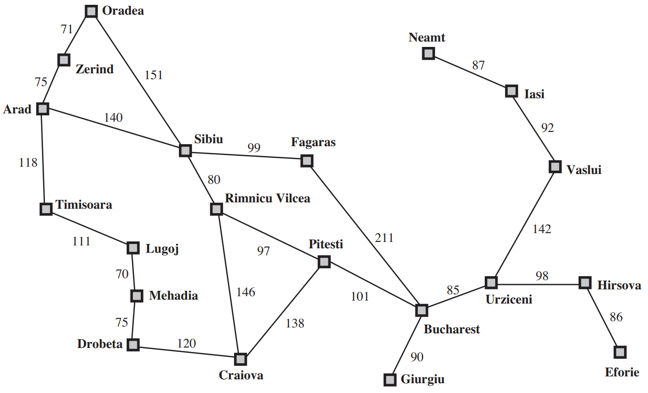 In the figure above we are given the graph of the romanian roadnetwork and asked to find the best route from Arad to Bucharest. Note that for applying A\* to more realistic example, you can use the [Open Street Maps](https://www.openstreetmap.org/) project and associated python libraries to produce much larger networks where the nodes may be cities or intersectionr or any other OSM tag (attribute).
For $h(s)$ we use the straightline distance heuristic, which we will call hSLD . If the goal is Bucharest, we need to
know the straight-line distances to Bucharest, which are shown below for all nodes in the graph.
In the figure above we are given the graph of the romanian roadnetwork and asked to find the best route from Arad to Bucharest. Note that for applying A\* to more realistic example, you can use the [Open Street Maps](https://www.openstreetmap.org/) project and associated python libraries to produce much larger networks where the nodes may be cities or intersectionr or any other OSM tag (attribute).
For $h(s)$ we use the straightline distance heuristic, which we will call hSLD . If the goal is Bucharest, we need to
know the straight-line distances to Bucharest, which are shown below for all nodes in the graph.
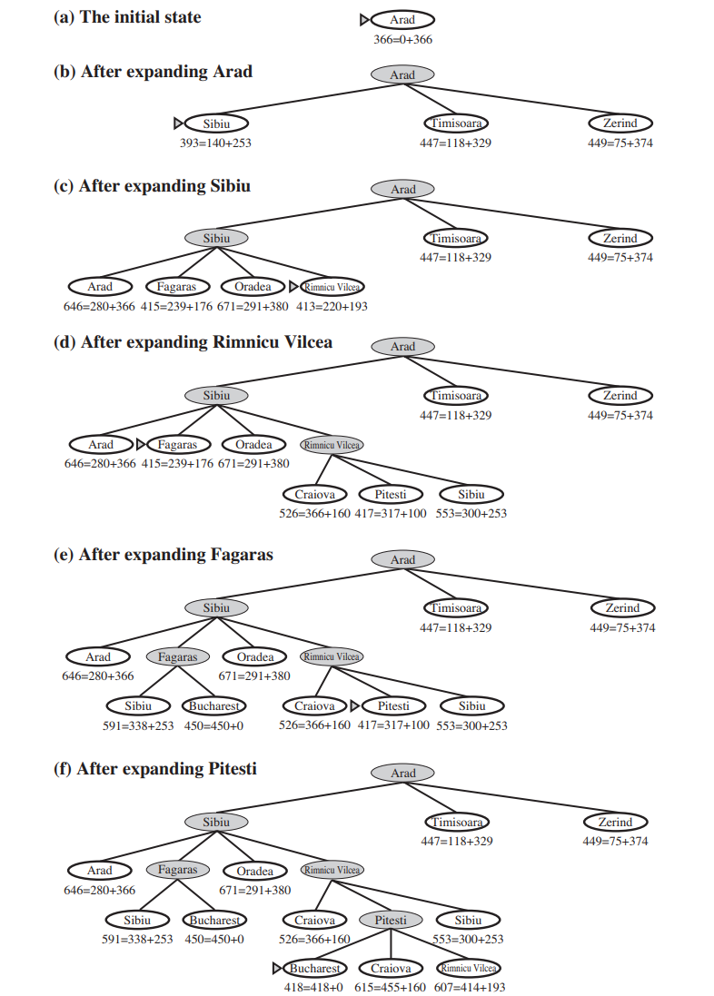
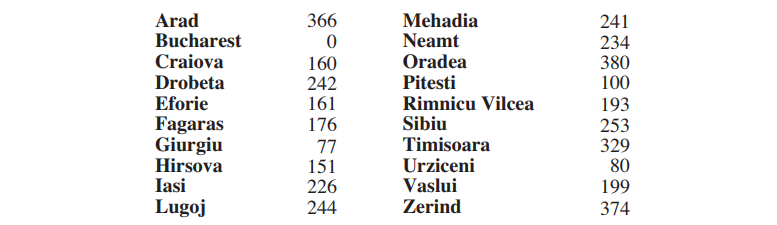 Notice that the values of $h(s)$ cannot be computed from the problem description itself. Moreover, it takes a certain amount of experience to know that $h(s)$ is correlated with actual road distances and is, therefore, a useful heuristic. Observe how the A\* algorithm behaves when using the heuristic $h(s)$ in the following figure.
 ## Demo
This [demo](https://qiao.github.io/PathFinding.js/visual/) is instructive of the various search algorithms we will cover here. You can introduce using your mouse obstacles in the canvas and see how the various search methods behave.
## Demo
This [demo](https://qiao.github.io/PathFinding.js/visual/) is instructive of the various search algorithms we will cover here. You can introduce using your mouse obstacles in the canvas and see how the various search methods behave.
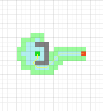 *$A^*$ algorithm demo . If the demo is not shown below, click on the link above. Define the gray wall and run all the search algorithms.*
We can clearly see the substantial difference in search speed and the beamforming-effect as soon as the wave (frontier) evaluates nodes where the heuristic (the Manhattan distance from the goal node) becomes dominant. Notice the difference between A\* and the UCS / Dijkstra's algorithm in the number of nodes that needed to be evaluated.
## Python Implementation
Open the A\* algorithm implementation in Google Colab to execute the code interactively.
## Other references
This is an [excellent overview](https://arxiv.org/abs/1504.05140) on how the principles of shortest path algorithms are applied in everyday applications such as Google maps directions. Practical implementation considerations are discussed for multi-modal route finding capabilities where the agent needs to find optimal routes while traversing multiple modes of transportation.
***
[Edit this page on GitHub](https://github.com/aegean-ai/eaia/edit/main/src/aiml-common/lectures/planning/global-planning/search/a-star/index.mdx) or [file an issue](https://github.com/aegean-ai/eaia/issues/new/choose).
*$A^*$ algorithm demo . If the demo is not shown below, click on the link above. Define the gray wall and run all the search algorithms.*
We can clearly see the substantial difference in search speed and the beamforming-effect as soon as the wave (frontier) evaluates nodes where the heuristic (the Manhattan distance from the goal node) becomes dominant. Notice the difference between A\* and the UCS / Dijkstra's algorithm in the number of nodes that needed to be evaluated.
## Python Implementation
Open the A\* algorithm implementation in Google Colab to execute the code interactively.
## Other references
This is an [excellent overview](https://arxiv.org/abs/1504.05140) on how the principles of shortest path algorithms are applied in everyday applications such as Google maps directions. Practical implementation considerations are discussed for multi-modal route finding capabilities where the agent needs to find optimal routes while traversing multiple modes of transportation.
***
[Edit this page on GitHub](https://github.com/aegean-ai/eaia/edit/main/src/aiml-common/lectures/planning/global-planning/search/a-star/index.mdx) or [file an issue](https://github.com/aegean-ai/eaia/issues/new/choose).