> ## Documentation Index
> Fetch the complete documentation index at: https://aegean.ai/llms.txt
> Use this file to discover all available pages before exploring further.
# Predicting the load of the electrical grid
> Fitting the noisy daily grid-load cycle with stochastic gradient descent on a ridge-regularized degree-9 polynomial, with lambda determined by an Optuna hyperparameter search.
 This example fits a degree-9 polynomial to a small sample of **real MISO grid load** by **stochastic gradient descent (SGD)** on the *regularized* empirical risk, the same ridge objective solved in closed form on the [linear regression](/aiml-common/lectures/regression/linear-regression) page. You reach the solution iteratively, and you determine the regularization strength $\lambda$ properly: an outer [Optuna](https://optuna.org/) hyperparameter search wrapped around the inner SGD fit selects the $\lambda^\ast$ that minimizes held-out error, tuned on this data rather than borrowed.
## The dataset
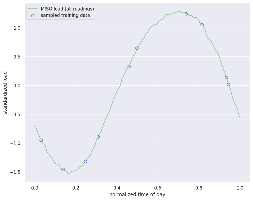
Read the daily grid-load cycle as your regression target: the input $x$ is normalized time across one day and the output $y$ is the system-wide load. You fetch one real day of MISO load from the gridstatus.io API, standardize it to zero mean and unit variance, and then **sample just ten readings** as the training set, deliberately small so a degree-9 polynomial can overfit it, the same regime the closed-form page studied. The remaining readings of the day are held out to score the regularization strength $\lambda$.
**MISO** is the **Midcontinent Independent System Operator**, the regional grid operator that runs the wholesale electricity market and balances generation against demand across 15 US states and the Canadian province of Manitoba. The daily rise-and-fall you are modeling is the real load pattern published on the [gridstatus.io MISO load dataset](https://www.gridstatus.io/datasets/miso_load); the figure below is one real day of it, pulled from the `miso_load` dataset via the gridstatus API.
This example fits a degree-9 polynomial to a small sample of **real MISO grid load** by **stochastic gradient descent (SGD)** on the *regularized* empirical risk, the same ridge objective solved in closed form on the [linear regression](/aiml-common/lectures/regression/linear-regression) page. You reach the solution iteratively, and you determine the regularization strength $\lambda$ properly: an outer [Optuna](https://optuna.org/) hyperparameter search wrapped around the inner SGD fit selects the $\lambda^\ast$ that minimizes held-out error, tuned on this data rather than borrowed.
## The dataset
Read the daily grid-load cycle as your regression target: the input $x$ is normalized time across one day and the output $y$ is the system-wide load. You fetch one real day of MISO load from the gridstatus.io API, standardize it to zero mean and unit variance, and then **sample just ten readings** as the training set, deliberately small so a degree-9 polynomial can overfit it, the same regime the closed-form page studied. The remaining readings of the day are held out to score the regularization strength $\lambda$.
**MISO** is the **Midcontinent Independent System Operator**, the regional grid operator that runs the wholesale electricity market and balances generation against demand across 15 US states and the Canadian province of Manitoba. The daily rise-and-fall you are modeling is the real load pattern published on the [gridstatus.io MISO load dataset](https://www.gridstatus.io/datasets/miso_load); the figure below is one real day of it, pulled from the `miso_load` dataset via the gridstatus API.
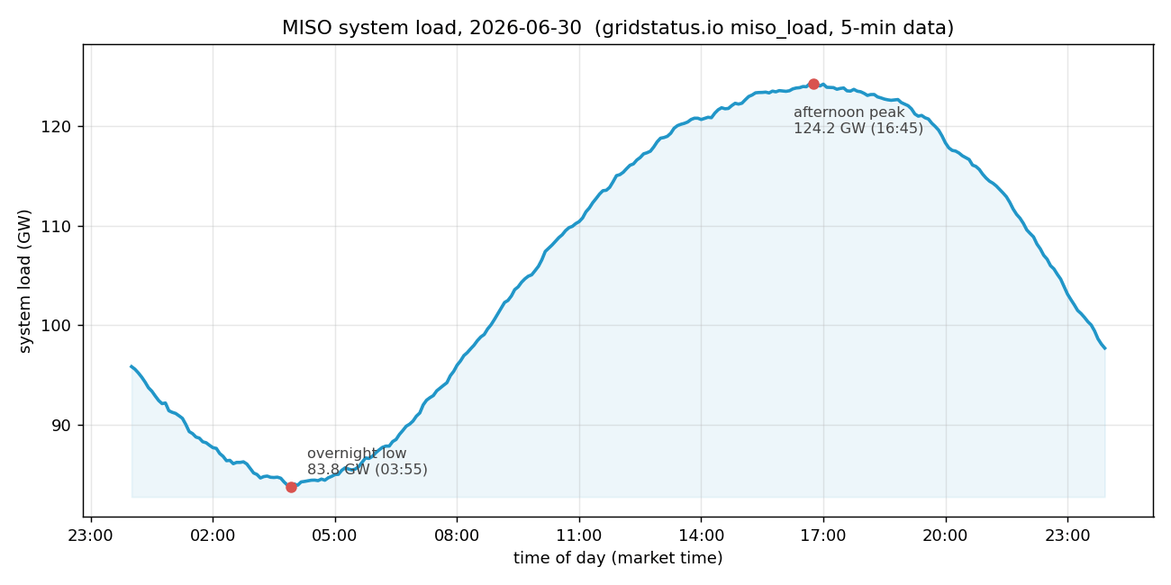 *Real MISO system load on 2026-06-30, five-minute data from the gridstatus.io `miso_load` dataset.*
Getting this prediction wrong is not academic. Operators schedule generation ahead of time against a load forecast, and the grid must match supply to demand second by second. Underpredict and too little generation is online to meet demand, forcing emergency purchases, frequency drops, and in the worst case load shedding (rolling blackouts); overpredict and expensive units are committed and paid for nothing. A model that generalizes poorly, one that chases the noise instead of the true demand curve, feeds a bad forecast straight into **grid stability**.
```python theme={null}
# Fetch one real day of MISO system load from the gridstatus.io API.
# GRIDSTATUS_API_KEY is read from the environment (.env); it is never hardcoded.
import logging
logging.getLogger("gridstatusio").setLevel(logging.WARNING)
load_dotenv()
client = GridStatusClient(os.environ["GRIDSTATUS_API_KEY"])
df = client.get_dataset(
dataset="miso_load",
start="2026-06-30",
end="2026-07-01",
timezone="market",
verbose=False,
)
t = pd.to_datetime(df["interval_start_local"])
secs = (t - t.min()).dt.total_seconds().to_numpy()
x_all = secs / secs.max() # normalized time of day in [0, 1]
load_gw = df["load"].to_numpy() / 1000.0 # system load in GW
# Standardize the target so the learning rate and lambda stay on a familiar (unit-variance) scale.
y_mean, y_std = load_gw.mean(), load_gw.std()
y_all = (load_gw - y_mean) / y_std
# A deliberately small training set (like the original ten-point toy set); the rest of the
# day is held out to score lambda.
rng = np.random.default_rng(1)
train_idx = np.sort(rng.choice(len(x_all), size=10, replace=False))
mask = np.ones(len(x_all), bool); mask[train_idx] = False
x_train, y_train = x_all[train_idx], y_all[train_idx]
x_val, y_val = x_all[mask], y_all[mask]
```
*Real MISO system load on 2026-06-30, five-minute data from the gridstatus.io `miso_load` dataset.*
Getting this prediction wrong is not academic. Operators schedule generation ahead of time against a load forecast, and the grid must match supply to demand second by second. Underpredict and too little generation is online to meet demand, forcing emergency purchases, frequency drops, and in the worst case load shedding (rolling blackouts); overpredict and expensive units are committed and paid for nothing. A model that generalizes poorly, one that chases the noise instead of the true demand curve, feeds a bad forecast straight into **grid stability**.
```python theme={null}
# Fetch one real day of MISO system load from the gridstatus.io API.
# GRIDSTATUS_API_KEY is read from the environment (.env); it is never hardcoded.
import logging
logging.getLogger("gridstatusio").setLevel(logging.WARNING)
load_dotenv()
client = GridStatusClient(os.environ["GRIDSTATUS_API_KEY"])
df = client.get_dataset(
dataset="miso_load",
start="2026-06-30",
end="2026-07-01",
timezone="market",
verbose=False,
)
t = pd.to_datetime(df["interval_start_local"])
secs = (t - t.min()).dt.total_seconds().to_numpy()
x_all = secs / secs.max() # normalized time of day in [0, 1]
load_gw = df["load"].to_numpy() / 1000.0 # system load in GW
# Standardize the target so the learning rate and lambda stay on a familiar (unit-variance) scale.
y_mean, y_std = load_gw.mean(), load_gw.std()
y_all = (load_gw - y_mean) / y_std
# A deliberately small training set (like the original ten-point toy set); the rest of the
# day is held out to score lambda.
rng = np.random.default_rng(1)
train_idx = np.sort(rng.choice(len(x_all), size=10, replace=False))
mask = np.ones(len(x_all), bool); mask[train_idx] = False
x_train, y_train = x_all[train_idx], y_all[train_idx]
x_val, y_val = x_all[mask], y_all[mask]
```
 ## Standardized polynomial features
The model is a degree-9 polynomial, $g(x;\boldsymbol{\theta}) = \bar{y} + \sum_{k=1}^{9}\theta_k\,\phi_k(x)$. Raw monomials $x, x^2, \dots, x^9$ on $[0,1]$ span many orders of magnitude, which makes the gradient steps lopsided and the penalty $\lambda\lVert\boldsymbol{\theta}\rVert^2$ act unevenly across coordinates. Standardizing each feature to zero mean and unit variance puts every coordinate on the same footing, so a single learning rate and a single $\lambda$ are meaningful and the value of $\lambda^\ast$ transfers directly from the closed-form page, which uses the same standardized features. The intercept is absorbed by centering the targets at $\bar{y}$.
```python theme={null}
M = 9
P_train = np.vander(x_train, M + 1, increasing=True)[:, 1:] # columns x^1 .. x^9
mu, sd = P_train.mean(0), P_train.std(0) + 1e-12
def featurize(xq):
P = np.vander(np.ravel(xq), M + 1, increasing=True)[:, 1:]
return (P - mu) / sd
Phi_train = featurize(x_train)
Phi_val = featurize(x_val) # the rest of the day, held out to score lambda
y_bar = y_train.mean() # intercept; SGD fits the centered residual
```
## The regularized objective and the SGD update
SGD minimizes the same ridge objective the closed-form page solves exactly, the sum of squared residuals plus an $\ell_2$ penalty,
$J(\boldsymbol{\theta}) = \sum_{i=1}^{n}\big(\boldsymbol{\phi}_i^{\top}\boldsymbol{\theta} - \tilde{y}_i\big)^2 + \lambda\lVert\boldsymbol{\theta}\rVert^2, \qquad \tilde{y}_i = y_i - \bar{y}.$
Its minimizer satisfies the normal equations $(\boldsymbol{\Phi}^{\top}\boldsymbol{\Phi} + \lambda\mathbf{I})\boldsymbol{\theta} = \boldsymbol{\Phi}^{\top}\tilde{\mathbf{y}}$, so using this convention makes $\lambda$ here identical to the closed-form $\lambda^\ast$. Each SGD step draws a mini-batch $\mathcal{B}$ of size $B$ and follows an unbiased estimate of the full gradient, scaling the batch sum by $n/B$:
$\boldsymbol{\theta} \leftarrow \boldsymbol{\theta} - \eta\Big(\tfrac{2n}{B}\,\boldsymbol{\Phi}_{\mathcal{B}}^{\top}(\boldsymbol{\Phi}_{\mathcal{B}}\boldsymbol{\theta} - \tilde{\mathbf{y}}_{\mathcal{B}}) + 2\lambda\boldsymbol{\theta}\Big).$
```python theme={null}
def sgd_fit(lam, lr=0.004, epochs=20000, batch_size=5, seed=0):
g = np.random.default_rng(seed)
yc = y_train - y_bar # centered target
n = len(y_train)
theta = np.zeros(M)
train_hist, val_hist = [], []
for _ in range(epochs):
order = g.permutation(n)
for s in range(0, n, batch_size):
b = order[s:s + batch_size]
err = Phi_train[b] @ theta - yc[b]
grad = (2 * n / len(b)) * (Phi_train[b].T @ err) + 2 * lam * theta
theta -= lr * grad
res = Phi_train @ theta - yc
train_hist.append(np.sum(res**2) + lam * np.sum(theta**2))
val_hist.append(np.mean((Phi_val @ theta + y_bar - y_val) ** 2))
return theta, np.array(train_hist), np.array(val_hist)
```
## Choosing $\lambda$ by nested hyperparameter search
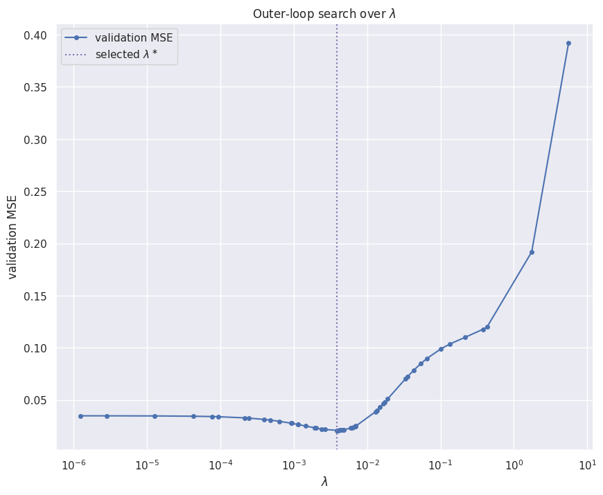
The regularization strength $\lambda$ is a hyperparameter: it cannot be read off the training loss, which always prefers $\lambda \to 0$ because less shrinkage fits the ten points more tightly. It has to be chosen by held-out performance, and that takes two nested loops.
* The **inner loop** is a full SGD fit of the degree-9 model at a fixed $\lambda$; it returns the validation error of the trained weights.
* The **outer loop** is the hyperparameter search. Optuna proposes a candidate $\lambda$ over a wide logarithmic range, reads back the validation error from the inner fit, and uses it to propose the next candidate, converging on the $\lambda^\ast$ that minimizes held-out error.
Nothing is borrowed here: $\lambda^\ast$ is determined from this grid-load sample.
```python theme={null}
import warnings
warnings.filterwarnings("ignore")
import optuna
optuna.logging.set_verbosity(optuna.logging.WARNING)
def objective(trial):
# outer loop proposes lambda over a wide range; inner loop is a full SGD fit
lam = trial.suggest_float("lambda", 1e-6, 1e1, log=True)
_, _, val_hist = sgd_fit(lam)
return float(np.mean(val_hist[-200:])) # validation MSE of the converged model
study = optuna.create_study(direction="minimize", sampler=optuna.samplers.TPESampler(seed=0))
study.optimize(objective, n_trials=50)
lambda_star = study.best_params["lambda"]
print(f"selected lambda* : {lambda_star:.2e}")
print(f"validation MSE at it : {study.best_value:.4f}")
```
```output theme={null}
selected lambda* : 3.89e-03
validation MSE at it : 0.0209
```
## Standardized polynomial features
The model is a degree-9 polynomial, $g(x;\boldsymbol{\theta}) = \bar{y} + \sum_{k=1}^{9}\theta_k\,\phi_k(x)$. Raw monomials $x, x^2, \dots, x^9$ on $[0,1]$ span many orders of magnitude, which makes the gradient steps lopsided and the penalty $\lambda\lVert\boldsymbol{\theta}\rVert^2$ act unevenly across coordinates. Standardizing each feature to zero mean and unit variance puts every coordinate on the same footing, so a single learning rate and a single $\lambda$ are meaningful and the value of $\lambda^\ast$ transfers directly from the closed-form page, which uses the same standardized features. The intercept is absorbed by centering the targets at $\bar{y}$.
```python theme={null}
M = 9
P_train = np.vander(x_train, M + 1, increasing=True)[:, 1:] # columns x^1 .. x^9
mu, sd = P_train.mean(0), P_train.std(0) + 1e-12
def featurize(xq):
P = np.vander(np.ravel(xq), M + 1, increasing=True)[:, 1:]
return (P - mu) / sd
Phi_train = featurize(x_train)
Phi_val = featurize(x_val) # the rest of the day, held out to score lambda
y_bar = y_train.mean() # intercept; SGD fits the centered residual
```
## The regularized objective and the SGD update
SGD minimizes the same ridge objective the closed-form page solves exactly, the sum of squared residuals plus an $\ell_2$ penalty,
$J(\boldsymbol{\theta}) = \sum_{i=1}^{n}\big(\boldsymbol{\phi}_i^{\top}\boldsymbol{\theta} - \tilde{y}_i\big)^2 + \lambda\lVert\boldsymbol{\theta}\rVert^2, \qquad \tilde{y}_i = y_i - \bar{y}.$
Its minimizer satisfies the normal equations $(\boldsymbol{\Phi}^{\top}\boldsymbol{\Phi} + \lambda\mathbf{I})\boldsymbol{\theta} = \boldsymbol{\Phi}^{\top}\tilde{\mathbf{y}}$, so using this convention makes $\lambda$ here identical to the closed-form $\lambda^\ast$. Each SGD step draws a mini-batch $\mathcal{B}$ of size $B$ and follows an unbiased estimate of the full gradient, scaling the batch sum by $n/B$:
$\boldsymbol{\theta} \leftarrow \boldsymbol{\theta} - \eta\Big(\tfrac{2n}{B}\,\boldsymbol{\Phi}_{\mathcal{B}}^{\top}(\boldsymbol{\Phi}_{\mathcal{B}}\boldsymbol{\theta} - \tilde{\mathbf{y}}_{\mathcal{B}}) + 2\lambda\boldsymbol{\theta}\Big).$
```python theme={null}
def sgd_fit(lam, lr=0.004, epochs=20000, batch_size=5, seed=0):
g = np.random.default_rng(seed)
yc = y_train - y_bar # centered target
n = len(y_train)
theta = np.zeros(M)
train_hist, val_hist = [], []
for _ in range(epochs):
order = g.permutation(n)
for s in range(0, n, batch_size):
b = order[s:s + batch_size]
err = Phi_train[b] @ theta - yc[b]
grad = (2 * n / len(b)) * (Phi_train[b].T @ err) + 2 * lam * theta
theta -= lr * grad
res = Phi_train @ theta - yc
train_hist.append(np.sum(res**2) + lam * np.sum(theta**2))
val_hist.append(np.mean((Phi_val @ theta + y_bar - y_val) ** 2))
return theta, np.array(train_hist), np.array(val_hist)
```
## Choosing $\lambda$ by nested hyperparameter search
The regularization strength $\lambda$ is a hyperparameter: it cannot be read off the training loss, which always prefers $\lambda \to 0$ because less shrinkage fits the ten points more tightly. It has to be chosen by held-out performance, and that takes two nested loops.
* The **inner loop** is a full SGD fit of the degree-9 model at a fixed $\lambda$; it returns the validation error of the trained weights.
* The **outer loop** is the hyperparameter search. Optuna proposes a candidate $\lambda$ over a wide logarithmic range, reads back the validation error from the inner fit, and uses it to propose the next candidate, converging on the $\lambda^\ast$ that minimizes held-out error.
Nothing is borrowed here: $\lambda^\ast$ is determined from this grid-load sample.
```python theme={null}
import warnings
warnings.filterwarnings("ignore")
import optuna
optuna.logging.set_verbosity(optuna.logging.WARNING)
def objective(trial):
# outer loop proposes lambda over a wide range; inner loop is a full SGD fit
lam = trial.suggest_float("lambda", 1e-6, 1e1, log=True)
_, _, val_hist = sgd_fit(lam)
return float(np.mean(val_hist[-200:])) # validation MSE of the converged model
study = optuna.create_study(direction="minimize", sampler=optuna.samplers.TPESampler(seed=0))
study.optimize(objective, n_trials=50)
lambda_star = study.best_params["lambda"]
print(f"selected lambda* : {lambda_star:.2e}")
print(f"validation MSE at it : {study.best_value:.4f}")
```
```output theme={null}
selected lambda* : 3.89e-03
validation MSE at it : 0.0209
```
 ## The selected fit
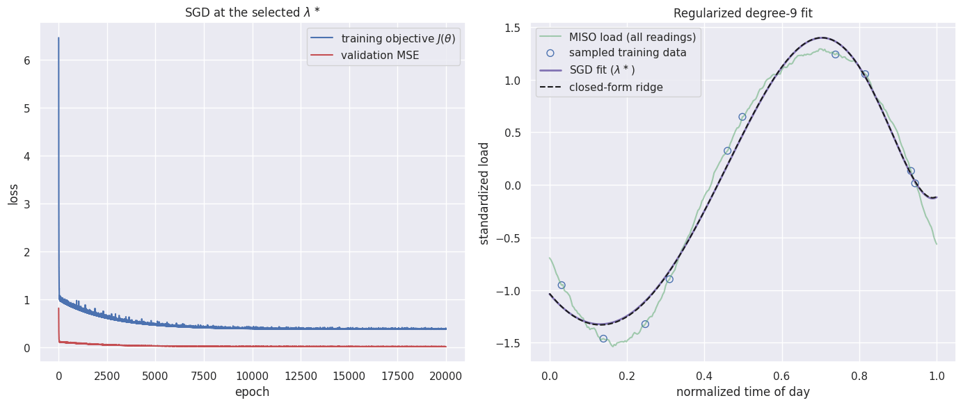
With $\lambda^\ast$ chosen by the search, fit the degree-9 model at that value and compare the iterative SGD solution against the closed-form ridge solution at the same $\lambda^\ast$. They should coincide: SGD is just an iterative route to the same regularized optimum.
```python theme={null}
theta_sgd, train_hist, val_hist = sgd_fit(lambda_star)
# closed-form ridge at the selected lambda, for comparison
theta_cf = np.linalg.solve(
Phi_train.T @ Phi_train + lambda_star * np.eye(M), Phi_train.T @ (y_train - y_bar))
xq = np.linspace(0, 1, 200)
gap = np.max(np.abs(featurize(xq) @ theta_sgd - featurize(xq) @ theta_cf))
print(f"validation MSE at lambda* : {val_hist[-1]:.4f}")
print(f"max |SGD - closed-form| over [0, 1] : {gap:.3f}")
```
```output theme={null}
validation MSE at lambda* : 0.0207
max |SGD - closed-form| over [0, 1] : 0.007
```
## The selected fit
With $\lambda^\ast$ chosen by the search, fit the degree-9 model at that value and compare the iterative SGD solution against the closed-form ridge solution at the same $\lambda^\ast$. They should coincide: SGD is just an iterative route to the same regularized optimum.
```python theme={null}
theta_sgd, train_hist, val_hist = sgd_fit(lambda_star)
# closed-form ridge at the selected lambda, for comparison
theta_cf = np.linalg.solve(
Phi_train.T @ Phi_train + lambda_star * np.eye(M), Phi_train.T @ (y_train - y_bar))
xq = np.linspace(0, 1, 200)
gap = np.max(np.abs(featurize(xq) @ theta_sgd - featurize(xq) @ theta_cf))
print(f"validation MSE at lambda* : {val_hist[-1]:.4f}")
print(f"max |SGD - closed-form| over [0, 1] : {gap:.3f}")
```
```output theme={null}
validation MSE at lambda* : 0.0207
max |SGD - closed-form| over [0, 1] : 0.007
```
 ## Takeaways
* Choosing $\lambda$ is **model selection by nested search**: an outer Optuna loop proposes $\lambda$ over a wide logarithmic range, and an inner SGD loop trains the degree-9 model at each candidate and reports its held-out error. The training loss alone cannot choose $\lambda$, it always prefers less shrinkage.
* SGD minimizes the **regularized** empirical risk: the penalty enters the gradient as $2\lambda\boldsymbol{\theta}$, shrinking the weights every step and curbing the degree-9 overfitting. At the selected $\lambda^\ast$ the iterative SGD fit and the direct closed-form solve reach the same regularized optimum.
* Standardizing both the features and the load makes a single $\lambda$ meaningful across every coordinate, so the outer search operates on a well-conditioned problem. Tuned from scratch on this real grid-load sample, the search settles near $4\times10^{-3}$, the same order as the $3.04\times10^{-3}$ the closed-form page found on a unit-variance sinusoid, an independent confirmation rather than a borrowed constant.
**Key references**: (Keskar et al., 2016; Bottou et al., 2016; Andrychowicz et al., 2016)
## References
* Andrychowicz, M., Denil, M., Gomez, S., Hoffman, M., Pfau, D., et al. (2016). *Learning to learn by gradient descent by gradient descent*.
* Bottou, L., Curtis, F., Nocedal, J. (2016). *Optimization Methods for Large-Scale Machine Learning*.
* Keskar, N., Mudigere, D., Nocedal, J., Smelyanskiy, M., Tang, P. (2016). *On Large-Batch Training for Deep Learning: Generalization Gap and Sharp Minima*.
***
[Edit this page on GitHub](https://github.com/aegean-ai/eaia/edit/main/src/aiml-common/lectures/regression/linear-regression/sgd/sgd_sinusoidal_dataset.mdx) or [file an issue](https://github.com/aegean-ai/eaia/issues/new/choose).
## Takeaways
* Choosing $\lambda$ is **model selection by nested search**: an outer Optuna loop proposes $\lambda$ over a wide logarithmic range, and an inner SGD loop trains the degree-9 model at each candidate and reports its held-out error. The training loss alone cannot choose $\lambda$, it always prefers less shrinkage.
* SGD minimizes the **regularized** empirical risk: the penalty enters the gradient as $2\lambda\boldsymbol{\theta}$, shrinking the weights every step and curbing the degree-9 overfitting. At the selected $\lambda^\ast$ the iterative SGD fit and the direct closed-form solve reach the same regularized optimum.
* Standardizing both the features and the load makes a single $\lambda$ meaningful across every coordinate, so the outer search operates on a well-conditioned problem. Tuned from scratch on this real grid-load sample, the search settles near $4\times10^{-3}$, the same order as the $3.04\times10^{-3}$ the closed-form page found on a unit-variance sinusoid, an independent confirmation rather than a borrowed constant.
**Key references**: (Keskar et al., 2016; Bottou et al., 2016; Andrychowicz et al., 2016)
## References
* Andrychowicz, M., Denil, M., Gomez, S., Hoffman, M., Pfau, D., et al. (2016). *Learning to learn by gradient descent by gradient descent*.
* Bottou, L., Curtis, F., Nocedal, J. (2016). *Optimization Methods for Large-Scale Machine Learning*.
* Keskar, N., Mudigere, D., Nocedal, J., Smelyanskiy, M., Tang, P. (2016). *On Large-Batch Training for Deep Learning: Generalization Gap and Sharp Minima*.
***
[Edit this page on GitHub](https://github.com/aegean-ai/eaia/edit/main/src/aiml-common/lectures/regression/linear-regression/sgd/sgd_sinusoidal_dataset.mdx) or [file an issue](https://github.com/aegean-ai/eaia/issues/new/choose).