> ## Documentation Index
> Fetch the complete documentation index at: https://aegean.ai/llms.txt
> Use this file to discover all available pages before exploring further.
# You Only Look Once (YOLO)
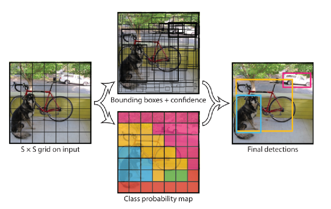 As shown in (see figure above), YOLOv1 partitions the input image into an $S\times S$ grid. If the center of an object falls in cell $i$, that cell is responsible for predicting it. Each grid cell outputs $B$ bounding-box hypotheses and one set of class probabilities over $C$ classes, yielding an $S\times S\times (B\cdot 5 + C)$ tensor. For VOC, $S=7$, $B=2$, $C=20 \Rightarrow 7\times7\times 30$.
Each bounding box prediction carries five numbers
$$
(x, y, w, h, \text{confidence}),
$$
where $(x,y)$ are the box-center offsets relative to the owning cell, and $(w,h)$ are normalized by image width/height. The confidence is intended to equal the IoU between the predicted box and the closest ground-truth box (and be $0$ when no object is present).
## Class-specific confidence at test time
At inference we combine per-cell conditional class probabilities with the per-box confidence to score each box for each class:
$$
\Pr(\text{Class}_i \mid \text{Object}) \cdot \Pr(\text{Object})\cdot \text{IoU}_{\text{pred}}^{\text{truth}}
\;=\;
\Pr(\text{Class}_i)\cdot \text{IoU}_{\text{pred}}^{\text{truth}}.
\tag{1}
$$
This produces class-specific confidence scores used before NMS.
## Network architecture and activations
As shown in (see figure above), YOLOv1 partitions the input image into an $S\times S$ grid. If the center of an object falls in cell $i$, that cell is responsible for predicting it. Each grid cell outputs $B$ bounding-box hypotheses and one set of class probabilities over $C$ classes, yielding an $S\times S\times (B\cdot 5 + C)$ tensor. For VOC, $S=7$, $B=2$, $C=20 \Rightarrow 7\times7\times 30$.
Each bounding box prediction carries five numbers
$$
(x, y, w, h, \text{confidence}),
$$
where $(x,y)$ are the box-center offsets relative to the owning cell, and $(w,h)$ are normalized by image width/height. The confidence is intended to equal the IoU between the predicted box and the closest ground-truth box (and be $0$ when no object is present).
## Class-specific confidence at test time
At inference we combine per-cell conditional class probabilities with the per-box confidence to score each box for each class:
$$
\Pr(\text{Class}_i \mid \text{Object}) \cdot \Pr(\text{Object})\cdot \text{IoU}_{\text{pred}}^{\text{truth}}
\;=\;
\Pr(\text{Class}_i)\cdot \text{IoU}_{\text{pred}}^{\text{truth}}.
\tag{1}
$$
This produces class-specific confidence scores used before NMS.
## Network architecture and activations
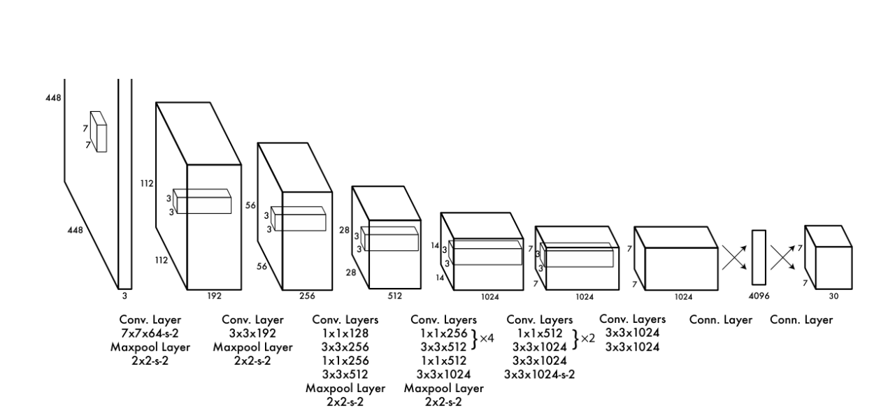 As shown in (see figure above), the detector is a single CNN: 24 conv layers + 2 fully-connected layers; early layers extract features, FC layers map to the $S\times S\times (B\cdot5+C)$ output. A fast variant reduces conv depth.
Final layer uses a linear activation; all others use leaky ReLU
$$
\phi(x)=
\begin{cases}
x, & x>0,\\
0.1x, & \text{otherwise.}
\end{cases}
\tag{2}
$$
Coordinates are normalized as described above.
## Training targets and responsibility
Because each cell predicts $B$ boxes, YOLO assigns “responsibility” to exactly one of the $B$ predictors for a given object: the predictor whose current box has the highest IoU with that object’s ground-truth. This specialization improves recall.
Consequence for targets:
* Only the responsible predictor for a cell/object receives coordinate and objectness regression targets for that object.
* The other predictor(s) in that cell are trained toward “no object” for confidence, reducing spurious positives.
That assignment happen per-iteration using the model’s current boxes.
## The multi-part loss
YOLOv1 optimizes a sum-squared error over location, size, objectness (confidence), and classification, with two balancing coefficients $\lambda_{\text{coord}}$ and $\lambda_{\text{noobj}}$. To de-emphasize scale sensitivity, the loss regresses $\sqrt{w},\sqrt{h}$ instead of $w,h$.
$$
\begin{aligned}
\mathcal{L} = \;&
\lambda_{\text{coord}}
\sum_{i=1}^{S^2}
\sum_{j=1}^{B}
\mathbf{1}^{\text{obj}}_{ij}
\Big[(x_i-\hat{x}_i)^2 + (y_i-\hat{y}_i)^2\Big] \\
&+ \lambda_{\text{coord}}
\sum_{i=1}^{S^2}
\sum_{j=1}^{B}
\mathbf{1}^{\text{obj}}_{ij}
\Big[\big(\sqrt{w_i}-\sqrt{\hat{w}_i}\big)^2 + \big(\sqrt{h_i}-\sqrt{\hat{h}_i}\big)^2\Big] \\
&+ \sum_{i=1}^{S^2}\sum_{j=1}^{B}
\mathbf{1}^{\text{obj}}_{ij}\big(C_i-\hat{C}_i\big)^2
+ \lambda_{\text{noobj}}
\sum_{i=1}^{S^2}\sum_{j=1}^{B}
\mathbf{1}^{\text{noobj}}_{ij}\big(C_i-\hat{C}_i\big)^2 \\
&+ \sum_{i=1}^{S^2}\mathbf{1}^{\text{obj}}_{i}
\sum_{c\in\mathcal{C}}\big(p_i(c)-\hat{p}_i(c)\big)^2.
\end{aligned}
$$
Here $\mathbf{1}^{\text{obj}}_{ij}=1$ iff predictor $j$ in cell $i$ is responsible for some object; $\mathbf{1}^{\text{noobj}}_{ij}=1$ for “no object” cases; $\lambda_{\text{coord}}=5$ and $\lambda_{\text{noobj}}=0.5$. Classification loss is applied only when a cell contains an object.
## Optimization details
Typical training recipe (VOC): \~135 epochs, batch size 64, momentum 0.9, weight decay $5\!\times\!10^{-4}$. LR warmup from $10^{-3}$ to $10^{-2}$, then $10^{-2}$ for 75 epochs, $10^{-3}$ for 30, $10^{-4}$ for 30. Regularization via dropout (rate 0.5 after first FC) and data augmentation (random scale/translation up to 20%, exposure/saturation jitters in HSV up to 1.5×).
## End-to-end inference
1. Preprocess: resize the image (e.g., to $448\times 448$) and forward once through the CNN.
2. Decode raw outputs:
* For each cell $i$ and predictor $j$: convert normalized $(x,y,w,h)$ to image coordinates; take the predicted confidence $C_{ij}$.
* Combine with class probabilities $p_i(c)$ using Eq. (1) to get class-specific scores $s_{ijc} = p_i(c)\cdot C_{ij}$.
3. Filter and suppress:
* Discard low-score boxes.
* Perform non-max suppression per class. While not as critical as in proposal-based pipelines, NMS adds \~2–3 mAP points by removing duplicates from neighboring cells.
## Strengths and limitations
* One-shot, global reasoning; extremely fast.
* Different error profile vs. R-CNN family (fewer background false positives, more localization errors).
* Limitations: fixed grid capacity (crowded small objects), coarse features due to downsampling, and sensitivity to small-box localization.
* Grid cell owns an object if the object’s center falls inside.
* Exactly one predictor per owned object learns its geometry (IoU-based responsibility).
* Confidence $=$ objectness $\times$ IoU; class probs are cell-level. Eq. (1) fuses them into a per-class score.
* Loss trades off localization, objectness, and classification with $\lambda_{\text{coord}},\lambda_{\text{noobj}}$; sizes use square-root to temper scale effects. Eq. (3).
## PyTorch sections
The following sections progressively build a complete YOLOv11 anchor-free detector from scratch in PyTorch.
COCO data loading, letterbox resizing, mosaic augmentation, and multi-scale target encoding for anchor-free detection.
Conv-BN-SiLU blocks, Bottleneck, C3k2 (CSP), SPPF, and the full backbone producing P3/P4/P5 features.
FPN top-down and PAN bottom-up feature aggregation, C2PSA attention, decoupled anchor-free head with DFL.
IoU variants (GIoU/DIoU/CIoU), Task-Aligned Learning, BCE + CIoU + DFL composite loss, training loop.
Prediction decoding, NMS from scratch, COCO mAP evaluation, Grad-CAM visualization.
## PyTorch reference
| PyTorch class | Description |
| -------------------------------------------------------------------------------------- | ------------------------------------------------------------------------------- |
| [`nn.Conv2d`](https://docs.pytorch.org/docs/2.12/generated/torch.nn.Conv2d.html) | Applies a 2D convolution over an input signal composed of several input planes. |
| [`nn.LeakyReLU`](https://docs.pytorch.org/docs/2.12/generated/torch.nn.LeakyReLU.html) | Applies the LeakyReLU function element-wise. |
| [`nn.MaxPool2d`](https://docs.pytorch.org/docs/2.12/generated/torch.nn.MaxPool2d.html) | Applies a 2D max pooling over an input signal composed of several input planes. |
| [`nn.Linear`](https://docs.pytorch.org/docs/2.12/generated/torch.nn.Linear.html) | Applies an affine linear transformation to the incoming data: $y = xA^T + b$. |
**Key references**: (Redmon et al., 2015; Redmon & Farhadi, 2016; Liu et al., 2015; Canziani et al., 2016; Godard et al., 2016)
## References
* Canziani, A., Paszke, A., Culurciello, E. (2016). *An Analysis of Deep Neural Network Models for Practical Applications*.
* Godard, C., Aodha, O., Brostow, G. (2016). *Unsupervised Monocular Depth Estimation with Left-Right Consistency*.
* Liu, W., Anguelov, D., Erhan, D., Szegedy, C., Reed, S., et al. (2015). *SSD: Single Shot MultiBox Detector*.
* Redmon, J., Divvala, S., Girshick, R., Farhadi, A. (2015). *You only look once: Unified, real-time object detection*.
* Redmon, J., Farhadi, A. (2016). *YOLO9000: Better, Faster, Stronger*.
***
[Edit this page on GitHub](https://github.com/aegean-ai/eaia/edit/main/src/aiml-common/lectures/scene-understanding/object-detection/yolo/introduction.mdx) or [file an issue](https://github.com/aegean-ai/eaia/issues/new/choose).
As shown in (see figure above), the detector is a single CNN: 24 conv layers + 2 fully-connected layers; early layers extract features, FC layers map to the $S\times S\times (B\cdot5+C)$ output. A fast variant reduces conv depth.
Final layer uses a linear activation; all others use leaky ReLU
$$
\phi(x)=
\begin{cases}
x, & x>0,\\
0.1x, & \text{otherwise.}
\end{cases}
\tag{2}
$$
Coordinates are normalized as described above.
## Training targets and responsibility
Because each cell predicts $B$ boxes, YOLO assigns “responsibility” to exactly one of the $B$ predictors for a given object: the predictor whose current box has the highest IoU with that object’s ground-truth. This specialization improves recall.
Consequence for targets:
* Only the responsible predictor for a cell/object receives coordinate and objectness regression targets for that object.
* The other predictor(s) in that cell are trained toward “no object” for confidence, reducing spurious positives.
That assignment happen per-iteration using the model’s current boxes.
## The multi-part loss
YOLOv1 optimizes a sum-squared error over location, size, objectness (confidence), and classification, with two balancing coefficients $\lambda_{\text{coord}}$ and $\lambda_{\text{noobj}}$. To de-emphasize scale sensitivity, the loss regresses $\sqrt{w},\sqrt{h}$ instead of $w,h$.
$$
\begin{aligned}
\mathcal{L} = \;&
\lambda_{\text{coord}}
\sum_{i=1}^{S^2}
\sum_{j=1}^{B}
\mathbf{1}^{\text{obj}}_{ij}
\Big[(x_i-\hat{x}_i)^2 + (y_i-\hat{y}_i)^2\Big] \\
&+ \lambda_{\text{coord}}
\sum_{i=1}^{S^2}
\sum_{j=1}^{B}
\mathbf{1}^{\text{obj}}_{ij}
\Big[\big(\sqrt{w_i}-\sqrt{\hat{w}_i}\big)^2 + \big(\sqrt{h_i}-\sqrt{\hat{h}_i}\big)^2\Big] \\
&+ \sum_{i=1}^{S^2}\sum_{j=1}^{B}
\mathbf{1}^{\text{obj}}_{ij}\big(C_i-\hat{C}_i\big)^2
+ \lambda_{\text{noobj}}
\sum_{i=1}^{S^2}\sum_{j=1}^{B}
\mathbf{1}^{\text{noobj}}_{ij}\big(C_i-\hat{C}_i\big)^2 \\
&+ \sum_{i=1}^{S^2}\mathbf{1}^{\text{obj}}_{i}
\sum_{c\in\mathcal{C}}\big(p_i(c)-\hat{p}_i(c)\big)^2.
\end{aligned}
$$
Here $\mathbf{1}^{\text{obj}}_{ij}=1$ iff predictor $j$ in cell $i$ is responsible for some object; $\mathbf{1}^{\text{noobj}}_{ij}=1$ for “no object” cases; $\lambda_{\text{coord}}=5$ and $\lambda_{\text{noobj}}=0.5$. Classification loss is applied only when a cell contains an object.
## Optimization details
Typical training recipe (VOC): \~135 epochs, batch size 64, momentum 0.9, weight decay $5\!\times\!10^{-4}$. LR warmup from $10^{-3}$ to $10^{-2}$, then $10^{-2}$ for 75 epochs, $10^{-3}$ for 30, $10^{-4}$ for 30. Regularization via dropout (rate 0.5 after first FC) and data augmentation (random scale/translation up to 20%, exposure/saturation jitters in HSV up to 1.5×).
## End-to-end inference
1. Preprocess: resize the image (e.g., to $448\times 448$) and forward once through the CNN.
2. Decode raw outputs:
* For each cell $i$ and predictor $j$: convert normalized $(x,y,w,h)$ to image coordinates; take the predicted confidence $C_{ij}$.
* Combine with class probabilities $p_i(c)$ using Eq. (1) to get class-specific scores $s_{ijc} = p_i(c)\cdot C_{ij}$.
3. Filter and suppress:
* Discard low-score boxes.
* Perform non-max suppression per class. While not as critical as in proposal-based pipelines, NMS adds \~2–3 mAP points by removing duplicates from neighboring cells.
## Strengths and limitations
* One-shot, global reasoning; extremely fast.
* Different error profile vs. R-CNN family (fewer background false positives, more localization errors).
* Limitations: fixed grid capacity (crowded small objects), coarse features due to downsampling, and sensitivity to small-box localization.
* Grid cell owns an object if the object’s center falls inside.
* Exactly one predictor per owned object learns its geometry (IoU-based responsibility).
* Confidence $=$ objectness $\times$ IoU; class probs are cell-level. Eq. (1) fuses them into a per-class score.
* Loss trades off localization, objectness, and classification with $\lambda_{\text{coord}},\lambda_{\text{noobj}}$; sizes use square-root to temper scale effects. Eq. (3).
## PyTorch sections
The following sections progressively build a complete YOLOv11 anchor-free detector from scratch in PyTorch.
COCO data loading, letterbox resizing, mosaic augmentation, and multi-scale target encoding for anchor-free detection.
Conv-BN-SiLU blocks, Bottleneck, C3k2 (CSP), SPPF, and the full backbone producing P3/P4/P5 features.
FPN top-down and PAN bottom-up feature aggregation, C2PSA attention, decoupled anchor-free head with DFL.
IoU variants (GIoU/DIoU/CIoU), Task-Aligned Learning, BCE + CIoU + DFL composite loss, training loop.
Prediction decoding, NMS from scratch, COCO mAP evaluation, Grad-CAM visualization.
## PyTorch reference
| PyTorch class | Description |
| -------------------------------------------------------------------------------------- | ------------------------------------------------------------------------------- |
| [`nn.Conv2d`](https://docs.pytorch.org/docs/2.12/generated/torch.nn.Conv2d.html) | Applies a 2D convolution over an input signal composed of several input planes. |
| [`nn.LeakyReLU`](https://docs.pytorch.org/docs/2.12/generated/torch.nn.LeakyReLU.html) | Applies the LeakyReLU function element-wise. |
| [`nn.MaxPool2d`](https://docs.pytorch.org/docs/2.12/generated/torch.nn.MaxPool2d.html) | Applies a 2D max pooling over an input signal composed of several input planes. |
| [`nn.Linear`](https://docs.pytorch.org/docs/2.12/generated/torch.nn.Linear.html) | Applies an affine linear transformation to the incoming data: $y = xA^T + b$. |
**Key references**: (Redmon et al., 2015; Redmon & Farhadi, 2016; Liu et al., 2015; Canziani et al., 2016; Godard et al., 2016)
## References
* Canziani, A., Paszke, A., Culurciello, E. (2016). *An Analysis of Deep Neural Network Models for Practical Applications*.
* Godard, C., Aodha, O., Brostow, G. (2016). *Unsupervised Monocular Depth Estimation with Left-Right Consistency*.
* Liu, W., Anguelov, D., Erhan, D., Szegedy, C., Reed, S., et al. (2015). *SSD: Single Shot MultiBox Detector*.
* Redmon, J., Divvala, S., Girshick, R., Farhadi, A. (2015). *You only look once: Unified, real-time object detection*.
* Redmon, J., Farhadi, A. (2016). *YOLO9000: Better, Faster, Stronger*.
***
[Edit this page on GitHub](https://github.com/aegean-ai/eaia/edit/main/src/aiml-common/lectures/scene-understanding/object-detection/yolo/introduction.mdx) or [file an issue](https://github.com/aegean-ai/eaia/issues/new/choose).