 *This section was written by [Ruimeng Yang](https://github.com/ruimengyang1) ([pull request #58](https://github.com/pantelis/eng-ai-agents/pull/58)), with help from an AI coding agent on the code. It reproduces the ideas of Chapter 39 of [*Foundations of Computer Vision*](https://visionbook.mit.edu/imaging_geometry.html) by Antonio Torralba, Phillip Isola, and William T. Freeman. The book's own figures are not reproduced here, because the book's license covers only the work in full; links point to them instead.*
This section follows the book's chapter on camera modeling and calibration. Each part pairs the book's explanation, with a link to its figure, with a small experiment in PyTorch that makes the geometry concrete: projection at several depths, the effect of the intrinsic parameters, backprojecting a pixel to a ray, camera pitch and the horizon, and a DLT calibration on synthetic data. It ends with a real calibration attempt on a measured meeting room. The [pinhole model](/aiml-common/lectures/sensor-models/cameras/pinhole-model), [camera calibration](/aiml-common/lectures/sensor-models/cameras/camera-calibration), and [Zhang's method](/aiml-common/lectures/sensor-models/cameras/zhang-calibration-alg) pages derive the same model and a practical calibration method in more depth.
```python theme={null}
import io
import json
import math
import random
from pathlib import Path
import matplotlib.pyplot as plt
import numpy as np
import torch
from matplotlib import colors as mcolors
from mpl_toolkits.mplot3d.art3d import Poly3DCollection
SEED = 39
random.seed(SEED)
np.random.seed(SEED)
_ = torch.manual_seed(SEED)
CHAPTER_DIR = Path("notebooks/CV/mit-foundations/chapter-39-camera-modeling")
if not CHAPTER_DIR.is_dir():
CHAPTER_DIR = Path(".")
PHOTO_URL = ("https://raw.githubusercontent.com/pantelis/eng-ai-agents/main/notebooks/CV/"
"mit-foundations/chapter-39-camera-modeling/assets/biaoding.jpg")
if not (CHAPTER_DIR / "assets" / "biaoding.jpg").exists():
import urllib.request
(CHAPTER_DIR / "assets").mkdir(parents=True, exist_ok=True)
urllib.request.urlretrieve(PHOTO_URL, CHAPTER_DIR / "assets" / "biaoding.jpg")
```
```python theme={null}
def homogenize(points: torch.Tensor) -> torch.Tensor:
ones = torch.ones((points.shape[0], 1), dtype=points.dtype)
return torch.cat([points, ones], dim=1)
def rotation_x(angle_deg: float) -> torch.Tensor:
t = math.radians(angle_deg)
c, s = math.cos(t), math.sin(t)
return torch.tensor([[1.0, 0.0, 0.0], [0.0, c, -s], [0.0, s, c]], dtype=torch.float64)
def rotation_y(angle_deg: float) -> torch.Tensor:
t = math.radians(angle_deg)
c, s = math.cos(t), math.sin(t)
return torch.tensor([[c, 0.0, s], [0.0, 1.0, 0.0], [-s, 0.0, c]], dtype=torch.float64)
def make_intrinsics(fx: float, fy: float, cx: float, cy: float) -> torch.Tensor:
return torch.tensor([[fx, 0.0, cx], [0.0, fy, cy], [0.0, 0.0, 1.0]], dtype=torch.float64)
def project_points(points_world: torch.Tensor, K: torch.Tensor, R: torch.Tensor, T: torch.Tensor) -> tuple[torch.Tensor, torch.Tensor]:
points_cam = (R @ (points_world - T).T).T
pixels_h = (K @ points_cam.T).T
pixels = pixels_h[:, :2] / pixels_h[:, 2:].clamp_min(1e-9)
return pixels, points_cam
def build_dlt_matrix(points_world: torch.Tensor, pixels: torch.Tensor) -> torch.Tensor:
rows = []
for P, p in zip(points_world, pixels, strict=True):
X, Y, Z = [float(v) for v in P]
x, y = [float(v) for v in p]
rows.append([-X, -Y, -Z, -1.0, 0.0, 0.0, 0.0, 0.0, x * X, x * Y, x * Z, x])
rows.append([0.0, 0.0, 0.0, 0.0, -X, -Y, -Z, -1.0, y * X, y * Y, y * Z, y])
return torch.tensor(rows, dtype=torch.float64)
def estimate_projection_matrix_dlt(points_world: torch.Tensor, pixels: torch.Tensor) -> torch.Tensor:
A = build_dlt_matrix(points_world, pixels)
_, _, vh = torch.linalg.svd(A)
M = vh[-1].reshape(3, 4)
return M / torch.linalg.norm(M)
def project_with_matrix(points_world: torch.Tensor, M: torch.Tensor) -> torch.Tensor:
Xh = homogenize(points_world).T
ph = (M @ Xh).T
return ph[:, :2] / ph[:, 2:3].clamp_min(1e-9)
```
```python theme={null}
def normalize_points_2d(points: np.ndarray) -> tuple[np.ndarray, np.ndarray]:
centroid = points.mean(axis=0)
mean_distance = np.linalg.norm(points - centroid, axis=1).mean()
scale = math.sqrt(2.0) / max(mean_distance, 1e-9)
T = np.array(
[
[scale, 0.0, -scale * centroid[0]],
[0.0, scale, -scale * centroid[1]],
[0.0, 0.0, 1.0],
],
dtype=np.float64,
)
points_h = np.concatenate([points, np.ones((points.shape[0], 1), dtype=np.float64)], axis=1)
normalized = (T @ points_h.T).T
return normalized[:, :2], T
def normalize_points_3d(points: np.ndarray) -> tuple[np.ndarray, np.ndarray]:
centroid = points.mean(axis=0)
mean_distance = np.linalg.norm(points - centroid, axis=1).mean()
scale = math.sqrt(3.0) / max(mean_distance, 1e-9)
U = np.array(
[
[scale, 0.0, 0.0, -scale * centroid[0]],
[0.0, scale, 0.0, -scale * centroid[1]],
[0.0, 0.0, scale, -scale * centroid[2]],
[0.0, 0.0, 0.0, 1.0],
],
dtype=np.float64,
)
points_h = np.concatenate([points, np.ones((points.shape[0], 1), dtype=np.float64)], axis=1)
normalized = (U @ points_h.T).T
return normalized[:, :3], U
def build_dlt_matrix_numpy(points_world: np.ndarray, pixels: np.ndarray) -> np.ndarray:
rows = []
for point_world, pixel in zip(points_world, pixels, strict=True):
X, Y, Z = point_world
u, v = pixel
rows.append([0.0, 0.0, 0.0, 0.0, -X, -Y, -Z, -1.0, v * X, v * Y, v * Z, v])
rows.append([X, Y, Z, 1.0, 0.0, 0.0, 0.0, 0.0, -u * X, -u * Y, -u * Z, -u])
return np.asarray(rows, dtype=np.float64)
def estimate_projection_matrix_normalized_dlt(points_world: np.ndarray, pixels: np.ndarray) -> tuple[np.ndarray, np.ndarray]:
normalized_pixels, T = normalize_points_2d(pixels)
normalized_world, U = normalize_points_3d(points_world)
A = build_dlt_matrix_numpy(normalized_world, normalized_pixels)
_, _, vh = np.linalg.svd(A)
projection_normalized = vh[-1].reshape(3, 4)
projection = np.linalg.inv(T) @ projection_normalized @ U
projection = projection / np.linalg.norm(projection[2, :3])
if projection[2, 3] > 0.0:
projection = -projection
return projection, A
def project_with_projection_matrix(points_world: np.ndarray, projection: np.ndarray) -> np.ndarray:
points_h = np.concatenate([points_world, np.ones((points_world.shape[0], 1), dtype=np.float64)], axis=1)
projected_h = (projection @ points_h.T).T
return projected_h[:, :2] / projected_h[:, 2:3]
def rq_decomposition(matrix: np.ndarray) -> tuple[np.ndarray, np.ndarray]:
q_matrix, r_matrix = np.linalg.qr(np.flipud(matrix).T)
r_matrix = np.flipud(r_matrix.T)
r_matrix = np.fliplr(r_matrix)
q_matrix = q_matrix.T
q_matrix = np.flipud(q_matrix)
diagonal_signs = np.where(np.diag(r_matrix) >= 0.0, 1.0, -1.0)
sign_matrix = np.diag(diagonal_signs)
r_matrix = r_matrix @ sign_matrix
q_matrix = sign_matrix @ q_matrix
if np.linalg.det(q_matrix) < 0.0:
sign_matrix = np.diag([1.0, 1.0, -1.0])
r_matrix = r_matrix @ sign_matrix
q_matrix = sign_matrix @ q_matrix
return r_matrix, q_matrix
def decompose_projection_matrix(projection: np.ndarray) -> tuple[np.ndarray, np.ndarray, np.ndarray, np.ndarray]:
camera_matrix = projection[:, :3]
intrinsics, rotation = rq_decomposition(camera_matrix)
sign_matrix = np.diag(
[
-1.0 if intrinsics[0, 0] < 0.0 else 1.0,
-1.0 if intrinsics[1, 1] < 0.0 else 1.0,
1.0,
]
)
intrinsics = intrinsics @ sign_matrix
rotation = sign_matrix @ rotation
intrinsics = intrinsics / intrinsics[2, 2]
translation = np.linalg.solve(intrinsics, projection[:, 3])
camera_center = -np.linalg.inv(camera_matrix) @ projection[:, 3]
return intrinsics, rotation, translation, camera_center
```
## Introduction
Chapter 39 shifts from the simple pinhole stories of earlier chapters to a more useful
camera model: one that can describe where the camera sits in the world, how it is
oriented, and how 3D points become pixels.
[Figure 39.1](https://visionbook.mit.edu/imaging_geometry.html#fig-world_and_camera_coordinates) in the book contrasts a camera-centered frame with a world-centered frame. It matters here because the whole chapter is about moving between those frames cleanly.
[Figure 39.2](https://visionbook.mit.edu/imaging_geometry.html) in the book shows the image whose geometry the chapter later models. It matters because calibration always connects a real picture back to a 3D scene.
The chapter's core idea is that calibration is about estimating the transformation from
world coordinates to image coordinates. Intrinsic parameters describe the camera itself.
Extrinsic parameters describe the camera's position and pose relative to the scene.
## 3D camera projections in homogeneous coordinates
Perspective projection contains a division by depth, which makes the equations awkward in
ordinary Euclidean coordinates. Homogeneous coordinates express the same mapping as
a matrix multiplication followed by a normalization step.
[Figure 39.3](https://visionbook.mit.edu/imaging_geometry.html#fig-pinholeGeometry2bis) in the book shows how a 3D point projects through a pinhole onto the image plane. It matters because homogeneous coordinates re-express this geometry in matrix form.
The point to keep in mind is that a 3D location `P = [X, Y, Z]^T` projects to image
coordinates roughly proportional to `X/Z` and `Y/Z`. Nearby points look larger because
dividing by a smaller depth amplifies the image coordinates.
### Parallel projection
Parallel projection removes that depth-dependent division. It is a simpler model that is
sometimes useful for distant scenes or for deriving intuition, but it does not capture
the foreshortening that real pinhole cameras produce.
```python theme={null}
z_values = torch.tensor([2.0, 4.0, 8.0], dtype=torch.float64)
xy = torch.tensor([1.2, 0.8], dtype=torch.float64)
principal_point = torch.tensor([0.0, 0.0], dtype=torch.float64)
perspective_points = torch.stack([xy / z for z in z_values])
parallel_point = xy.clone()
```
*This section was written by [Ruimeng Yang](https://github.com/ruimengyang1) ([pull request #58](https://github.com/pantelis/eng-ai-agents/pull/58)), with help from an AI coding agent on the code. It reproduces the ideas of Chapter 39 of [*Foundations of Computer Vision*](https://visionbook.mit.edu/imaging_geometry.html) by Antonio Torralba, Phillip Isola, and William T. Freeman. The book's own figures are not reproduced here, because the book's license covers only the work in full; links point to them instead.*
This section follows the book's chapter on camera modeling and calibration. Each part pairs the book's explanation, with a link to its figure, with a small experiment in PyTorch that makes the geometry concrete: projection at several depths, the effect of the intrinsic parameters, backprojecting a pixel to a ray, camera pitch and the horizon, and a DLT calibration on synthetic data. It ends with a real calibration attempt on a measured meeting room. The [pinhole model](/aiml-common/lectures/sensor-models/cameras/pinhole-model), [camera calibration](/aiml-common/lectures/sensor-models/cameras/camera-calibration), and [Zhang's method](/aiml-common/lectures/sensor-models/cameras/zhang-calibration-alg) pages derive the same model and a practical calibration method in more depth.
```python theme={null}
import io
import json
import math
import random
from pathlib import Path
import matplotlib.pyplot as plt
import numpy as np
import torch
from matplotlib import colors as mcolors
from mpl_toolkits.mplot3d.art3d import Poly3DCollection
SEED = 39
random.seed(SEED)
np.random.seed(SEED)
_ = torch.manual_seed(SEED)
CHAPTER_DIR = Path("notebooks/CV/mit-foundations/chapter-39-camera-modeling")
if not CHAPTER_DIR.is_dir():
CHAPTER_DIR = Path(".")
PHOTO_URL = ("https://raw.githubusercontent.com/pantelis/eng-ai-agents/main/notebooks/CV/"
"mit-foundations/chapter-39-camera-modeling/assets/biaoding.jpg")
if not (CHAPTER_DIR / "assets" / "biaoding.jpg").exists():
import urllib.request
(CHAPTER_DIR / "assets").mkdir(parents=True, exist_ok=True)
urllib.request.urlretrieve(PHOTO_URL, CHAPTER_DIR / "assets" / "biaoding.jpg")
```
```python theme={null}
def homogenize(points: torch.Tensor) -> torch.Tensor:
ones = torch.ones((points.shape[0], 1), dtype=points.dtype)
return torch.cat([points, ones], dim=1)
def rotation_x(angle_deg: float) -> torch.Tensor:
t = math.radians(angle_deg)
c, s = math.cos(t), math.sin(t)
return torch.tensor([[1.0, 0.0, 0.0], [0.0, c, -s], [0.0, s, c]], dtype=torch.float64)
def rotation_y(angle_deg: float) -> torch.Tensor:
t = math.radians(angle_deg)
c, s = math.cos(t), math.sin(t)
return torch.tensor([[c, 0.0, s], [0.0, 1.0, 0.0], [-s, 0.0, c]], dtype=torch.float64)
def make_intrinsics(fx: float, fy: float, cx: float, cy: float) -> torch.Tensor:
return torch.tensor([[fx, 0.0, cx], [0.0, fy, cy], [0.0, 0.0, 1.0]], dtype=torch.float64)
def project_points(points_world: torch.Tensor, K: torch.Tensor, R: torch.Tensor, T: torch.Tensor) -> tuple[torch.Tensor, torch.Tensor]:
points_cam = (R @ (points_world - T).T).T
pixels_h = (K @ points_cam.T).T
pixels = pixels_h[:, :2] / pixels_h[:, 2:].clamp_min(1e-9)
return pixels, points_cam
def build_dlt_matrix(points_world: torch.Tensor, pixels: torch.Tensor) -> torch.Tensor:
rows = []
for P, p in zip(points_world, pixels, strict=True):
X, Y, Z = [float(v) for v in P]
x, y = [float(v) for v in p]
rows.append([-X, -Y, -Z, -1.0, 0.0, 0.0, 0.0, 0.0, x * X, x * Y, x * Z, x])
rows.append([0.0, 0.0, 0.0, 0.0, -X, -Y, -Z, -1.0, y * X, y * Y, y * Z, y])
return torch.tensor(rows, dtype=torch.float64)
def estimate_projection_matrix_dlt(points_world: torch.Tensor, pixels: torch.Tensor) -> torch.Tensor:
A = build_dlt_matrix(points_world, pixels)
_, _, vh = torch.linalg.svd(A)
M = vh[-1].reshape(3, 4)
return M / torch.linalg.norm(M)
def project_with_matrix(points_world: torch.Tensor, M: torch.Tensor) -> torch.Tensor:
Xh = homogenize(points_world).T
ph = (M @ Xh).T
return ph[:, :2] / ph[:, 2:3].clamp_min(1e-9)
```
```python theme={null}
def normalize_points_2d(points: np.ndarray) -> tuple[np.ndarray, np.ndarray]:
centroid = points.mean(axis=0)
mean_distance = np.linalg.norm(points - centroid, axis=1).mean()
scale = math.sqrt(2.0) / max(mean_distance, 1e-9)
T = np.array(
[
[scale, 0.0, -scale * centroid[0]],
[0.0, scale, -scale * centroid[1]],
[0.0, 0.0, 1.0],
],
dtype=np.float64,
)
points_h = np.concatenate([points, np.ones((points.shape[0], 1), dtype=np.float64)], axis=1)
normalized = (T @ points_h.T).T
return normalized[:, :2], T
def normalize_points_3d(points: np.ndarray) -> tuple[np.ndarray, np.ndarray]:
centroid = points.mean(axis=0)
mean_distance = np.linalg.norm(points - centroid, axis=1).mean()
scale = math.sqrt(3.0) / max(mean_distance, 1e-9)
U = np.array(
[
[scale, 0.0, 0.0, -scale * centroid[0]],
[0.0, scale, 0.0, -scale * centroid[1]],
[0.0, 0.0, scale, -scale * centroid[2]],
[0.0, 0.0, 0.0, 1.0],
],
dtype=np.float64,
)
points_h = np.concatenate([points, np.ones((points.shape[0], 1), dtype=np.float64)], axis=1)
normalized = (U @ points_h.T).T
return normalized[:, :3], U
def build_dlt_matrix_numpy(points_world: np.ndarray, pixels: np.ndarray) -> np.ndarray:
rows = []
for point_world, pixel in zip(points_world, pixels, strict=True):
X, Y, Z = point_world
u, v = pixel
rows.append([0.0, 0.0, 0.0, 0.0, -X, -Y, -Z, -1.0, v * X, v * Y, v * Z, v])
rows.append([X, Y, Z, 1.0, 0.0, 0.0, 0.0, 0.0, -u * X, -u * Y, -u * Z, -u])
return np.asarray(rows, dtype=np.float64)
def estimate_projection_matrix_normalized_dlt(points_world: np.ndarray, pixels: np.ndarray) -> tuple[np.ndarray, np.ndarray]:
normalized_pixels, T = normalize_points_2d(pixels)
normalized_world, U = normalize_points_3d(points_world)
A = build_dlt_matrix_numpy(normalized_world, normalized_pixels)
_, _, vh = np.linalg.svd(A)
projection_normalized = vh[-1].reshape(3, 4)
projection = np.linalg.inv(T) @ projection_normalized @ U
projection = projection / np.linalg.norm(projection[2, :3])
if projection[2, 3] > 0.0:
projection = -projection
return projection, A
def project_with_projection_matrix(points_world: np.ndarray, projection: np.ndarray) -> np.ndarray:
points_h = np.concatenate([points_world, np.ones((points_world.shape[0], 1), dtype=np.float64)], axis=1)
projected_h = (projection @ points_h.T).T
return projected_h[:, :2] / projected_h[:, 2:3]
def rq_decomposition(matrix: np.ndarray) -> tuple[np.ndarray, np.ndarray]:
q_matrix, r_matrix = np.linalg.qr(np.flipud(matrix).T)
r_matrix = np.flipud(r_matrix.T)
r_matrix = np.fliplr(r_matrix)
q_matrix = q_matrix.T
q_matrix = np.flipud(q_matrix)
diagonal_signs = np.where(np.diag(r_matrix) >= 0.0, 1.0, -1.0)
sign_matrix = np.diag(diagonal_signs)
r_matrix = r_matrix @ sign_matrix
q_matrix = sign_matrix @ q_matrix
if np.linalg.det(q_matrix) < 0.0:
sign_matrix = np.diag([1.0, 1.0, -1.0])
r_matrix = r_matrix @ sign_matrix
q_matrix = sign_matrix @ q_matrix
return r_matrix, q_matrix
def decompose_projection_matrix(projection: np.ndarray) -> tuple[np.ndarray, np.ndarray, np.ndarray, np.ndarray]:
camera_matrix = projection[:, :3]
intrinsics, rotation = rq_decomposition(camera_matrix)
sign_matrix = np.diag(
[
-1.0 if intrinsics[0, 0] < 0.0 else 1.0,
-1.0 if intrinsics[1, 1] < 0.0 else 1.0,
1.0,
]
)
intrinsics = intrinsics @ sign_matrix
rotation = sign_matrix @ rotation
intrinsics = intrinsics / intrinsics[2, 2]
translation = np.linalg.solve(intrinsics, projection[:, 3])
camera_center = -np.linalg.inv(camera_matrix) @ projection[:, 3]
return intrinsics, rotation, translation, camera_center
```
## Introduction
Chapter 39 shifts from the simple pinhole stories of earlier chapters to a more useful
camera model: one that can describe where the camera sits in the world, how it is
oriented, and how 3D points become pixels.
[Figure 39.1](https://visionbook.mit.edu/imaging_geometry.html#fig-world_and_camera_coordinates) in the book contrasts a camera-centered frame with a world-centered frame. It matters here because the whole chapter is about moving between those frames cleanly.
[Figure 39.2](https://visionbook.mit.edu/imaging_geometry.html) in the book shows the image whose geometry the chapter later models. It matters because calibration always connects a real picture back to a 3D scene.
The chapter's core idea is that calibration is about estimating the transformation from
world coordinates to image coordinates. Intrinsic parameters describe the camera itself.
Extrinsic parameters describe the camera's position and pose relative to the scene.
## 3D camera projections in homogeneous coordinates
Perspective projection contains a division by depth, which makes the equations awkward in
ordinary Euclidean coordinates. Homogeneous coordinates express the same mapping as
a matrix multiplication followed by a normalization step.
[Figure 39.3](https://visionbook.mit.edu/imaging_geometry.html#fig-pinholeGeometry2bis) in the book shows how a 3D point projects through a pinhole onto the image plane. It matters because homogeneous coordinates re-express this geometry in matrix form.
The point to keep in mind is that a 3D location `P = [X, Y, Z]^T` projects to image
coordinates roughly proportional to `X/Z` and `Y/Z`. Nearby points look larger because
dividing by a smaller depth amplifies the image coordinates.
### Parallel projection
Parallel projection removes that depth-dependent division. It is a simpler model that is
sometimes useful for distant scenes or for deriving intuition, but it does not capture
the foreshortening that real pinhole cameras produce.
```python theme={null}
z_values = torch.tensor([2.0, 4.0, 8.0], dtype=torch.float64)
xy = torch.tensor([1.2, 0.8], dtype=torch.float64)
principal_point = torch.tensor([0.0, 0.0], dtype=torch.float64)
perspective_points = torch.stack([xy / z for z in z_values])
parallel_point = xy.clone()
```
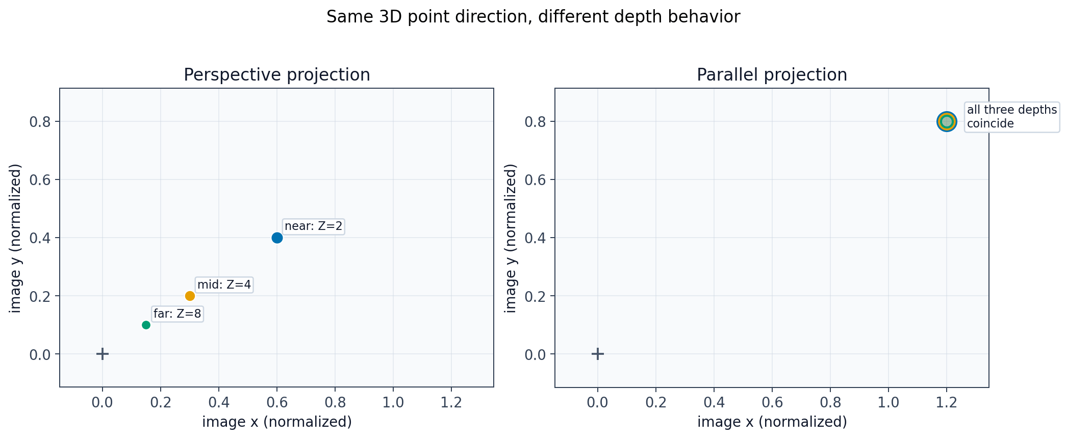 **Supplemental visualization.**
The figure projects the same lateral 3D point at three depths using both perspective and parallel projection. The perspective panel shrinks image coordinates with increasing depth, while the parallel panel keeps them fixed. That is the key geometric difference between perspective and parallel projection.
## Camera-intrinsic parameters
Intrinsic parameters describe how the camera turns rays into pixels. In practice, this
includes focal scaling, the principal point, and sometimes unequal pixel scales, skew,
or lens distortion.
### From meters to pixels
[Figure 39.4](https://visionbook.mit.edu/imaging_geometry.html#fig-pinhole_and_sensor) in the book shows how focal length, sensor width, and pixel sampling connect physical geometry to image coordinates. It matters because intrinsic calibration lives in that conversion.
The intrinsic matrix converts camera-plane coordinates into pixel
coordinates. The chapter uses `a` and `b` for horizontal and vertical focal scaling, and
`(c_x, c_y)` for the principal point.
[Figure 39.5](https://visionbook.mit.edu/imaging_geometry.html#fig-conventions) in the book compares common image-coordinate conventions. It matters because sign choices and origin placement change how you write the intrinsic matrix.
In code, it is worth being explicit about conventions: image origins, axis directions,
and sign choices all affect the exact matrix form even when the geometry is the same.
### From pixels to rays
[Figure 39.6](https://visionbook.mit.edu/imaging_geometry.html#fig-coordinate_systems_ray) in the book shows that a single pixel defines a whole 3D ray, not a unique 3D point. It matters because depth is what turns that ray back into a specific scene location.
Backprojection reverses the forward camera map only up to a ray. If a pixel is known and
the depth is unknown, there are infinitely many 3D points consistent with that pixel.
### A simple, although unreliable, calibration method
[Figure 39.7](https://visionbook.mit.edu/imaging_geometry.html#fig-simple_calibration) in the book groups the physical setup and the captured chessboard image. It matters because the chapter first introduces calibration as a measurement problem before presenting more general estimation methods.
This sanity-check method uses a known target, a measured distance, and the apparent size
of the target in the image to estimate focal scaling. It is useful for intuition, but it
ignores many practical effects such as distortion and imperfect alignment.
### Other camera parameters
Real cameras may also need skew terms, separate horizontal and vertical pixel scales, and
especially distortion correction. In practice, radial distortion is often the first extra
effect that visibly breaks the simplest pinhole model.
```python theme={null}
pattern_xy = torch.tensor(
[
[-0.9, -0.9], [0.0, -0.9], [0.9, -0.9],
[-0.9, 0.0], [0.0, 0.0], [0.9, 0.0],
[-0.9, 0.9], [0.0, 0.9], [0.9, 0.9],
],
dtype=torch.float64,
)
pattern_depth = torch.full((pattern_xy.shape[0], 1), 4.5, dtype=torch.float64)
pattern_3d = torch.cat([pattern_xy, pattern_depth], dim=1)
K_base = make_intrinsics(560.0, 560.0, 320.0, 240.0)
K_focal = make_intrinsics(780.0, 780.0, 320.0, 240.0)
K_shift = make_intrinsics(560.0, 560.0, 390.0, 185.0)
R_eye = torch.eye(3, dtype=torch.float64)
T_zero = torch.zeros(3, dtype=torch.float64)
baseline_pixels, _ = project_points(pattern_3d, K_base, R_eye, T_zero)
focal_pixels, _ = project_points(pattern_3d, K_focal, R_eye, T_zero)
shift_pixels, _ = project_points(pattern_3d, K_shift, R_eye, T_zero)
principal_base = torch.tensor([320.0, 240.0], dtype=torch.float64)
principal_shift = torch.tensor([390.0, 185.0], dtype=torch.float64)
all_points = torch.vstack([baseline_pixels, focal_pixels, shift_pixels, principal_base.unsqueeze(0), principal_shift.unsqueeze(0)])
pad_x = 0.08 * float(all_points[:, 0].max() - all_points[:, 0].min()) + 10.0
pad_y = 0.08 * float(all_points[:, 1].max() - all_points[:, 1].min()) + 10.0
xlim = (float(all_points[:, 0].min()) - pad_x, float(all_points[:, 0].max()) + pad_x)
y_top = float(all_points[:, 1].min()) - pad_y
y_bottom = float(all_points[:, 1].max()) + pad_y
```
**Supplemental visualization.**
The figure projects the same lateral 3D point at three depths using both perspective and parallel projection. The perspective panel shrinks image coordinates with increasing depth, while the parallel panel keeps them fixed. That is the key geometric difference between perspective and parallel projection.
## Camera-intrinsic parameters
Intrinsic parameters describe how the camera turns rays into pixels. In practice, this
includes focal scaling, the principal point, and sometimes unequal pixel scales, skew,
or lens distortion.
### From meters to pixels
[Figure 39.4](https://visionbook.mit.edu/imaging_geometry.html#fig-pinhole_and_sensor) in the book shows how focal length, sensor width, and pixel sampling connect physical geometry to image coordinates. It matters because intrinsic calibration lives in that conversion.
The intrinsic matrix converts camera-plane coordinates into pixel
coordinates. The chapter uses `a` and `b` for horizontal and vertical focal scaling, and
`(c_x, c_y)` for the principal point.
[Figure 39.5](https://visionbook.mit.edu/imaging_geometry.html#fig-conventions) in the book compares common image-coordinate conventions. It matters because sign choices and origin placement change how you write the intrinsic matrix.
In code, it is worth being explicit about conventions: image origins, axis directions,
and sign choices all affect the exact matrix form even when the geometry is the same.
### From pixels to rays
[Figure 39.6](https://visionbook.mit.edu/imaging_geometry.html#fig-coordinate_systems_ray) in the book shows that a single pixel defines a whole 3D ray, not a unique 3D point. It matters because depth is what turns that ray back into a specific scene location.
Backprojection reverses the forward camera map only up to a ray. If a pixel is known and
the depth is unknown, there are infinitely many 3D points consistent with that pixel.
### A simple, although unreliable, calibration method
[Figure 39.7](https://visionbook.mit.edu/imaging_geometry.html#fig-simple_calibration) in the book groups the physical setup and the captured chessboard image. It matters because the chapter first introduces calibration as a measurement problem before presenting more general estimation methods.
This sanity-check method uses a known target, a measured distance, and the apparent size
of the target in the image to estimate focal scaling. It is useful for intuition, but it
ignores many practical effects such as distortion and imperfect alignment.
### Other camera parameters
Real cameras may also need skew terms, separate horizontal and vertical pixel scales, and
especially distortion correction. In practice, radial distortion is often the first extra
effect that visibly breaks the simplest pinhole model.
```python theme={null}
pattern_xy = torch.tensor(
[
[-0.9, -0.9], [0.0, -0.9], [0.9, -0.9],
[-0.9, 0.0], [0.0, 0.0], [0.9, 0.0],
[-0.9, 0.9], [0.0, 0.9], [0.9, 0.9],
],
dtype=torch.float64,
)
pattern_depth = torch.full((pattern_xy.shape[0], 1), 4.5, dtype=torch.float64)
pattern_3d = torch.cat([pattern_xy, pattern_depth], dim=1)
K_base = make_intrinsics(560.0, 560.0, 320.0, 240.0)
K_focal = make_intrinsics(780.0, 780.0, 320.0, 240.0)
K_shift = make_intrinsics(560.0, 560.0, 390.0, 185.0)
R_eye = torch.eye(3, dtype=torch.float64)
T_zero = torch.zeros(3, dtype=torch.float64)
baseline_pixels, _ = project_points(pattern_3d, K_base, R_eye, T_zero)
focal_pixels, _ = project_points(pattern_3d, K_focal, R_eye, T_zero)
shift_pixels, _ = project_points(pattern_3d, K_shift, R_eye, T_zero)
principal_base = torch.tensor([320.0, 240.0], dtype=torch.float64)
principal_shift = torch.tensor([390.0, 185.0], dtype=torch.float64)
all_points = torch.vstack([baseline_pixels, focal_pixels, shift_pixels, principal_base.unsqueeze(0), principal_shift.unsqueeze(0)])
pad_x = 0.08 * float(all_points[:, 0].max() - all_points[:, 0].min()) + 10.0
pad_y = 0.08 * float(all_points[:, 1].max() - all_points[:, 1].min()) + 10.0
xlim = (float(all_points[:, 0].min()) - pad_x, float(all_points[:, 0].max()) + pad_x)
y_top = float(all_points[:, 1].min()) - pad_y
y_bottom = float(all_points[:, 1].max()) + pad_y
```
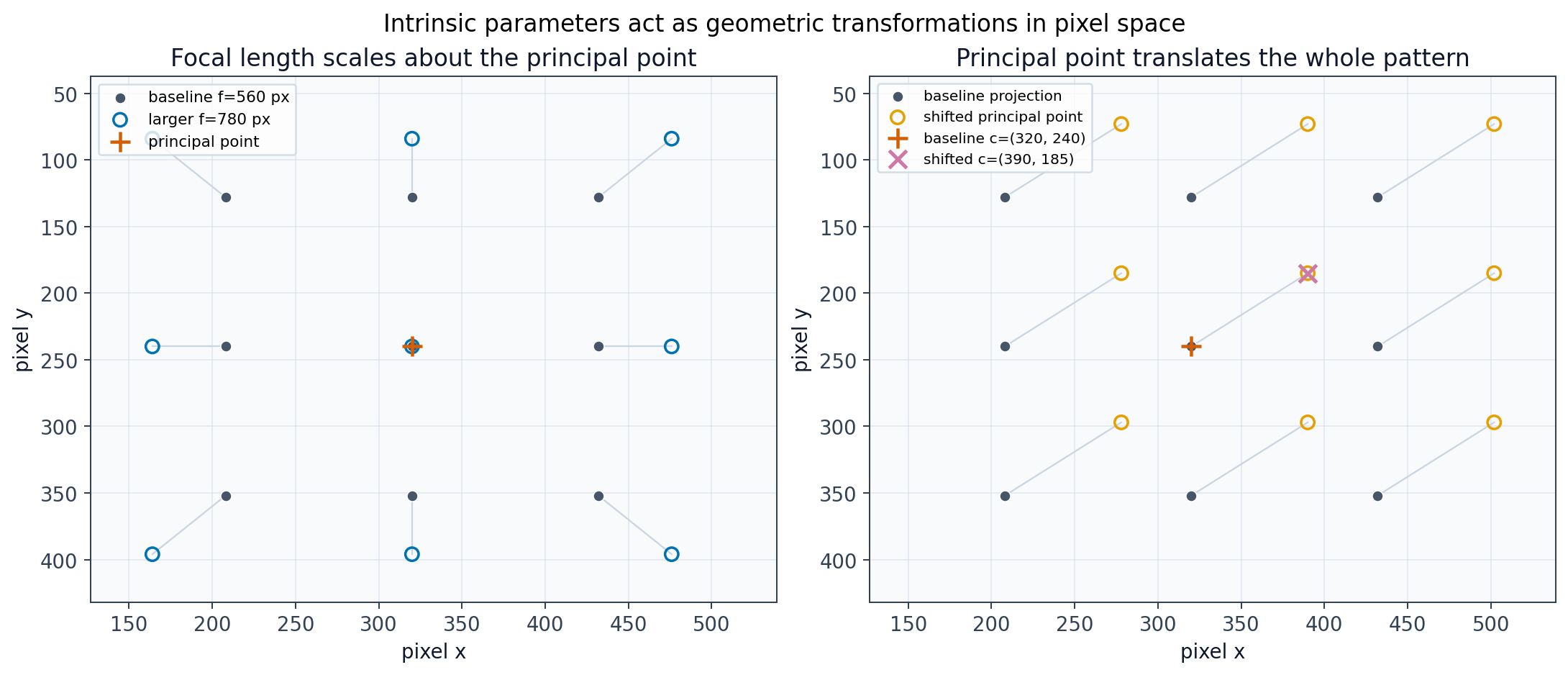 **Computational reconstruction related to Figure 39.4 of the book.**
The figure projects the same nine 3D points while changing either focal scaling or the principal point. Larger focal length magnifies the image, while changing `(c_x, c_y)` translates all projected points together. Those are two of the central effects encoded by the intrinsic matrix.
```python theme={null}
pixel = torch.tensor([220.0, -120.0], dtype=torch.float64)
focal = 500.0
depths = torch.tensor([1.5, 3.0, 5.0], dtype=torch.float64)
plane_depth = 1.0
pixel_on_plane = torch.tensor([pixel[0] / focal, pixel[1] / focal, plane_depth], dtype=torch.float64)
ray_dir = pixel_on_plane.clone()
ray_points = depths.unsqueeze(1) * ray_dir.unsqueeze(0)
plane_w, plane_h = 0.9, 0.7
plane_vertices = [
[-plane_w, -plane_h, plane_depth],
[ plane_w, -plane_h, plane_depth],
[ plane_w, plane_h, plane_depth],
[-plane_w, plane_h, plane_depth],
]
```
**Computational reconstruction related to Figure 39.4 of the book.**
The figure projects the same nine 3D points while changing either focal scaling or the principal point. Larger focal length magnifies the image, while changing `(c_x, c_y)` translates all projected points together. Those are two of the central effects encoded by the intrinsic matrix.
```python theme={null}
pixel = torch.tensor([220.0, -120.0], dtype=torch.float64)
focal = 500.0
depths = torch.tensor([1.5, 3.0, 5.0], dtype=torch.float64)
plane_depth = 1.0
pixel_on_plane = torch.tensor([pixel[0] / focal, pixel[1] / focal, plane_depth], dtype=torch.float64)
ray_dir = pixel_on_plane.clone()
ray_points = depths.unsqueeze(1) * ray_dir.unsqueeze(0)
plane_w, plane_h = 0.9, 0.7
plane_vertices = [
[-plane_w, -plane_h, plane_depth],
[ plane_w, -plane_h, plane_depth],
[ plane_w, plane_h, plane_depth],
[-plane_w, plane_h, plane_depth],
]
```
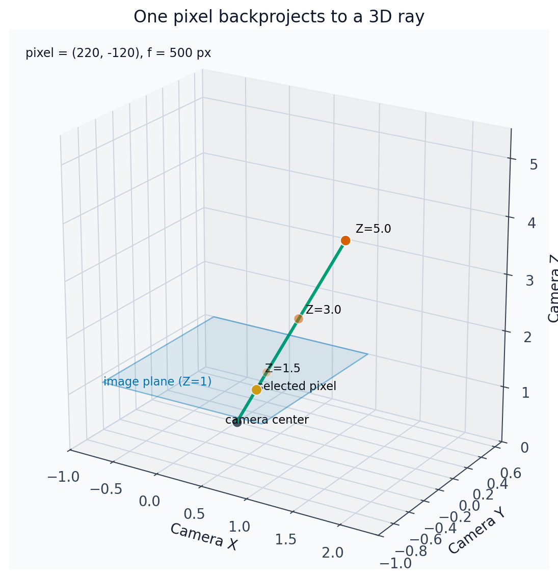 **Computational reconstruction related to Figure 39.6 of the book.**
The code chooses one pixel direction and sampled three depths along its backprojected ray. The computed points all correspond to the same image location, which is exactly why a pixel alone is insufficient to recover a unique 3D point.
## Camera-extrinsic parameters
Extrinsic parameters answer a different question from intrinsics: where is the camera in
the world, and how is it rotated relative to the world frame?
[Figure 39.8](https://visionbook.mit.edu/imaging_geometry.html#fig-camera_calibration) in the book shows the extrinsic relationship between the world frame and the camera frame. It matters because `R` and `T` explain where the camera is and how it is oriented.
The chapter writes this mapping as a rotation followed by a translation in homogeneous
coordinates. Once points are expressed in the camera frame, the intrinsic matrix can
project them into the image.
## Full camera model
[Figure 39.9](https://visionbook.mit.edu/imaging_geometry.html#fig-summary_camera_projection) in the book summarizes the full pipeline from world coordinates to camera coordinates to pixels. It matters because the projection matrix combines all of those steps.
The full projection matrix composes intrinsics with extrinsics. In compact notation, the
camera matrix is often written as `M = K [R | -RT]`.
## A few concrete examples
[Figure 39.10](https://visionbook.mit.edu/imaging_geometry.html#fig-camera_calibration_scenarios) in the book collects the concrete camera-pose cases discussed in the chapter. It matters because the same matrix model can represent all of them.
The chapter then walks through level cameras, tilted cameras, and more structured ground
scenes to show how pose affects the final image equations.
[Figure 39.11](https://visionbook.mit.edu/imaging_geometry.html#fig-horizon_heads) in the book shows a practical horizon cue in a level camera. It matters because camera orientation leaves visible traces in ordinary photographs.
[Figure 39.12](https://visionbook.mit.edu/imaging_geometry.html#fig-sketch_eyes_location) in the book sketches why equal-height points can line up in the image despite being at different depths. It matters because the horizon is a geometric consequence of camera pose.
[Figure 39.13](https://visionbook.mit.edu/imaging_geometry.html#fig-low_and_high_horizon) in the book groups two photos taken with different camera tilt angles. It matters because changing the camera pitch shifts the horizon line in a predictable way.
A helpful way to read these examples is to ask which quantities stay fixed when the
camera tilts or translates. Horizon-line motion is especially useful because it gives a
visible signature of camera pitch.
```python theme={null}
K = make_intrinsics(500.0, 500.0, 0.0, 0.0)
T = torch.tensor([0.0, 1.6, 0.0], dtype=torch.float64)
pitches = [0.0, 15.0]
ground_x = torch.linspace(-4.5, 4.5, 10, dtype=torch.float64)
ground_z = torch.linspace(6.0, 18.0, 7, dtype=torch.float64)
ground_points = torch.tensor([[float(x), 0.0, float(z)] for z in ground_z for x in ground_x], dtype=torch.float64)
horizon_points = torch.tensor([[float(x), float(T[1]), 1500.0] for x in torch.linspace(-6.0, 6.0, 13, dtype=torch.float64)], dtype=torch.float64)
reference_people = torch.tensor([[-3.0, float(T[1]), 8.0], [0.0, float(T[1]), 12.0], [3.0, float(T[1]), 16.0]], dtype=torch.float64)
```
**Computational reconstruction related to Figure 39.6 of the book.**
The code chooses one pixel direction and sampled three depths along its backprojected ray. The computed points all correspond to the same image location, which is exactly why a pixel alone is insufficient to recover a unique 3D point.
## Camera-extrinsic parameters
Extrinsic parameters answer a different question from intrinsics: where is the camera in
the world, and how is it rotated relative to the world frame?
[Figure 39.8](https://visionbook.mit.edu/imaging_geometry.html#fig-camera_calibration) in the book shows the extrinsic relationship between the world frame and the camera frame. It matters because `R` and `T` explain where the camera is and how it is oriented.
The chapter writes this mapping as a rotation followed by a translation in homogeneous
coordinates. Once points are expressed in the camera frame, the intrinsic matrix can
project them into the image.
## Full camera model
[Figure 39.9](https://visionbook.mit.edu/imaging_geometry.html#fig-summary_camera_projection) in the book summarizes the full pipeline from world coordinates to camera coordinates to pixels. It matters because the projection matrix combines all of those steps.
The full projection matrix composes intrinsics with extrinsics. In compact notation, the
camera matrix is often written as `M = K [R | -RT]`.
## A few concrete examples
[Figure 39.10](https://visionbook.mit.edu/imaging_geometry.html#fig-camera_calibration_scenarios) in the book collects the concrete camera-pose cases discussed in the chapter. It matters because the same matrix model can represent all of them.
The chapter then walks through level cameras, tilted cameras, and more structured ground
scenes to show how pose affects the final image equations.
[Figure 39.11](https://visionbook.mit.edu/imaging_geometry.html#fig-horizon_heads) in the book shows a practical horizon cue in a level camera. It matters because camera orientation leaves visible traces in ordinary photographs.
[Figure 39.12](https://visionbook.mit.edu/imaging_geometry.html#fig-sketch_eyes_location) in the book sketches why equal-height points can line up in the image despite being at different depths. It matters because the horizon is a geometric consequence of camera pose.
[Figure 39.13](https://visionbook.mit.edu/imaging_geometry.html#fig-low_and_high_horizon) in the book groups two photos taken with different camera tilt angles. It matters because changing the camera pitch shifts the horizon line in a predictable way.
A helpful way to read these examples is to ask which quantities stay fixed when the
camera tilts or translates. Horizon-line motion is especially useful because it gives a
visible signature of camera pitch.
```python theme={null}
K = make_intrinsics(500.0, 500.0, 0.0, 0.0)
T = torch.tensor([0.0, 1.6, 0.0], dtype=torch.float64)
pitches = [0.0, 15.0]
ground_x = torch.linspace(-4.5, 4.5, 10, dtype=torch.float64)
ground_z = torch.linspace(6.0, 18.0, 7, dtype=torch.float64)
ground_points = torch.tensor([[float(x), 0.0, float(z)] for z in ground_z for x in ground_x], dtype=torch.float64)
horizon_points = torch.tensor([[float(x), float(T[1]), 1500.0] for x in torch.linspace(-6.0, 6.0, 13, dtype=torch.float64)], dtype=torch.float64)
reference_people = torch.tensor([[-3.0, float(T[1]), 8.0], [0.0, float(T[1]), 12.0], [3.0, float(T[1]), 16.0]], dtype=torch.float64)
```
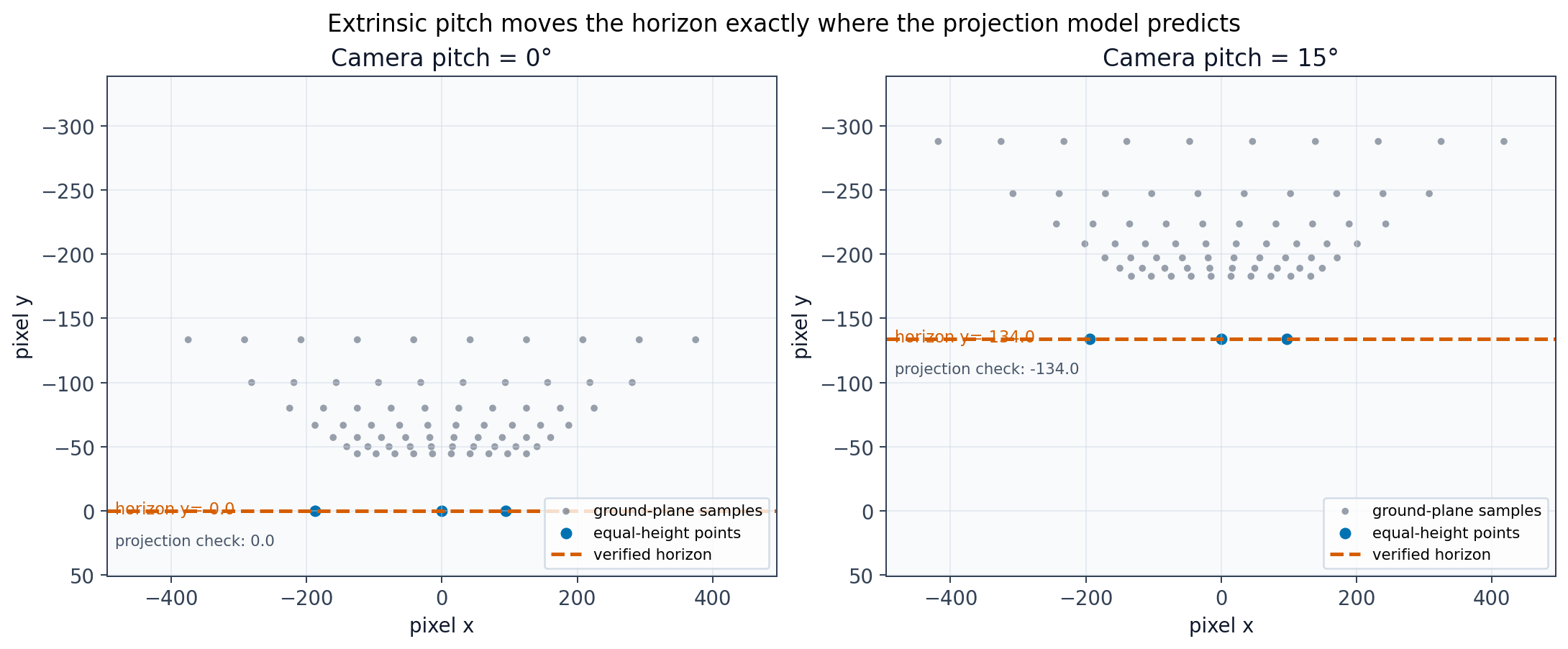 **Supplemental visualization.**
The figure projects a small set of equal-height scene points with a level camera and with a 15 degree downward pitch. The dashed line marks the numerically verified horizon height `y_h = -f tan(theta)` under the convention used here, `P_C = R(P_W - T)`, and the displayed image coordinates use the standard image convention where `y` increases downward.
## Camera calibration
Calibration estimates the mapping from known 3D scene points to observed 2D image
points. The chapter first introduces a linear estimate of the projection matrix and then
discusses how to recover more interpretable intrinsic and extrinsic parameters.
### Direct linear transform
DLT solves for a projection matrix by stacking linear equations from several 3D-to-2D
correspondences. The result is determined only up to an overall scale, which is fine for
projective geometry.
### Recovering intrinsic and extrinsic camera parameters
Once a projection matrix has been estimated, it still has to be factored into camera
intrinsics and pose. Conceptually, this means separating the left `3x3` calibration part
from the world-to-camera pose terms.
### Multiplane calibration method
Multiplane calibration uses several views of a known planar target to stabilize the
parameter estimates. This is closer to what practical camera-calibration toolkits do.
### Nonlinear optimization by minimizing reprojection error
[Figure 39.14](https://visionbook.mit.edu/imaging_geometry.html#fig-reprojection_error) in the book shows reprojection error directly on the image plane. It matters because nonlinear refinement usually optimizes camera parameters by minimizing this quantity.
Linear estimates are often only the starting point. A better model is usually obtained by
refining parameters to minimize the distance between observed image points and predicted
image points.
### A toy example
[Figure 39.15](https://visionbook.mit.edu/imaging_geometry.html#fig-office_measurements) in the book shows the real office scene used in the toy calibration example. It matters because the later 3D annotations are grounded in these measurements.
[Figure 39.16](https://visionbook.mit.edu/imaging_geometry.html#fig-office_correspondences_img) in the book pairs image observations with measured 3D coordinates. It matters because calibration needs matched 3D scene points and 2D image points.
[Figure 39.17](https://visionbook.mit.edu/imaging_geometry.html#fig-result_toymodel_3dscene_and_estimated_camera) in the book visualizes the inferred camera location from several viewpoints. It matters because a good calibration should produce a physically plausible camera pose.
The office example shows the whole calibration story end to end: measure some 3D
positions, annotate the corresponding image points, estimate the camera, and then inspect
whether the result is plausible.
```python theme={null}
world_points = torch.tensor(
[
[-1.5, -0.5, 4.0],
[-0.5, -0.2, 5.2],
[ 0.6, -0.3, 6.4],
[ 1.4, 0.1, 7.0],
[-1.2, 0.7, 5.0],
[-0.2, 0.9, 6.0],
[ 0.8, 1.1, 6.8],
[ 1.6, 0.8, 8.0],
],
dtype=torch.float64,
)
K_true = make_intrinsics(820.0, 790.0, 320.0, 240.0)
R_true = rotation_y(8.0) @ rotation_x(-12.0)
T_true = torch.tensor([0.3, 0.6, -0.4], dtype=torch.float64)
observed_pixels, _ = project_points(world_points, K_true, R_true, T_true)
noisy_pixels = observed_pixels + 0.8 * torch.tensor(
[[0.5, -0.3], [-0.4, 0.2], [0.1, 0.4], [0.3, -0.5], [-0.2, 0.6], [0.4, -0.1], [-0.3, -0.2], [0.2, 0.3]],
dtype=torch.float64,
)
M_est = estimate_projection_matrix_dlt(world_points, noisy_pixels)
reproj_clean = project_with_matrix(world_points, M_est)
reproj_error = torch.linalg.norm(reproj_clean - noisy_pixels, dim=1)
A = build_dlt_matrix(world_points, noisy_pixels)
A_display = torch.log10(A.abs() + 1e-6).numpy()
vector_scale = 18.0
```
**Supplemental visualization.**
The figure projects a small set of equal-height scene points with a level camera and with a 15 degree downward pitch. The dashed line marks the numerically verified horizon height `y_h = -f tan(theta)` under the convention used here, `P_C = R(P_W - T)`, and the displayed image coordinates use the standard image convention where `y` increases downward.
## Camera calibration
Calibration estimates the mapping from known 3D scene points to observed 2D image
points. The chapter first introduces a linear estimate of the projection matrix and then
discusses how to recover more interpretable intrinsic and extrinsic parameters.
### Direct linear transform
DLT solves for a projection matrix by stacking linear equations from several 3D-to-2D
correspondences. The result is determined only up to an overall scale, which is fine for
projective geometry.
### Recovering intrinsic and extrinsic camera parameters
Once a projection matrix has been estimated, it still has to be factored into camera
intrinsics and pose. Conceptually, this means separating the left `3x3` calibration part
from the world-to-camera pose terms.
### Multiplane calibration method
Multiplane calibration uses several views of a known planar target to stabilize the
parameter estimates. This is closer to what practical camera-calibration toolkits do.
### Nonlinear optimization by minimizing reprojection error
[Figure 39.14](https://visionbook.mit.edu/imaging_geometry.html#fig-reprojection_error) in the book shows reprojection error directly on the image plane. It matters because nonlinear refinement usually optimizes camera parameters by minimizing this quantity.
Linear estimates are often only the starting point. A better model is usually obtained by
refining parameters to minimize the distance between observed image points and predicted
image points.
### A toy example
[Figure 39.15](https://visionbook.mit.edu/imaging_geometry.html#fig-office_measurements) in the book shows the real office scene used in the toy calibration example. It matters because the later 3D annotations are grounded in these measurements.
[Figure 39.16](https://visionbook.mit.edu/imaging_geometry.html#fig-office_correspondences_img) in the book pairs image observations with measured 3D coordinates. It matters because calibration needs matched 3D scene points and 2D image points.
[Figure 39.17](https://visionbook.mit.edu/imaging_geometry.html#fig-result_toymodel_3dscene_and_estimated_camera) in the book visualizes the inferred camera location from several viewpoints. It matters because a good calibration should produce a physically plausible camera pose.
The office example shows the whole calibration story end to end: measure some 3D
positions, annotate the corresponding image points, estimate the camera, and then inspect
whether the result is plausible.
```python theme={null}
world_points = torch.tensor(
[
[-1.5, -0.5, 4.0],
[-0.5, -0.2, 5.2],
[ 0.6, -0.3, 6.4],
[ 1.4, 0.1, 7.0],
[-1.2, 0.7, 5.0],
[-0.2, 0.9, 6.0],
[ 0.8, 1.1, 6.8],
[ 1.6, 0.8, 8.0],
],
dtype=torch.float64,
)
K_true = make_intrinsics(820.0, 790.0, 320.0, 240.0)
R_true = rotation_y(8.0) @ rotation_x(-12.0)
T_true = torch.tensor([0.3, 0.6, -0.4], dtype=torch.float64)
observed_pixels, _ = project_points(world_points, K_true, R_true, T_true)
noisy_pixels = observed_pixels + 0.8 * torch.tensor(
[[0.5, -0.3], [-0.4, 0.2], [0.1, 0.4], [0.3, -0.5], [-0.2, 0.6], [0.4, -0.1], [-0.3, -0.2], [0.2, 0.3]],
dtype=torch.float64,
)
M_est = estimate_projection_matrix_dlt(world_points, noisy_pixels)
reproj_clean = project_with_matrix(world_points, M_est)
reproj_error = torch.linalg.norm(reproj_clean - noisy_pixels, dim=1)
A = build_dlt_matrix(world_points, noisy_pixels)
A_display = torch.log10(A.abs() + 1e-6).numpy()
vector_scale = 18.0
```
 ```python theme={null}
print("Estimated projection matrix (normalized):")
print(M_est)
print(f"Mean reprojection error: {reproj_error.mean().item():.3f} px")
```
```output theme={null}
Estimated projection matrix (normalized):
tensor([[ 5.9194e-01, -7.8249e-02, 3.4478e-01, -7.8726e-02],
[-4.3553e-02, 5.6133e-01, 3.2921e-01, -3.0505e-01],
[-1.3287e-04, -1.7602e-04, 7.8526e-04, 3.0855e-04]],
dtype=torch.float64)
Mean reprojection error: 0.248 px
```
**Computational reconstruction related to Figure 39.14 of the book.**
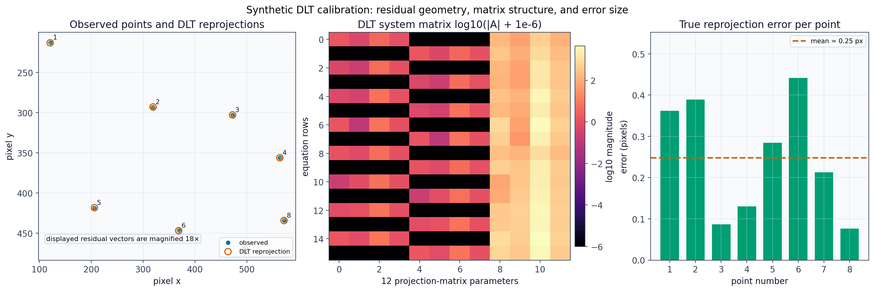
The code generates synthetic 3D points, projects them with a known camera, adds small image noise, builds the DLT linear system, and estimates a projection matrix up to scale. The left panel compares observed and predicted image points, the center panel shows the stacked DLT system, and the right panel summarizes reprojection error.
### A real calibration attempt: a measured meeting room
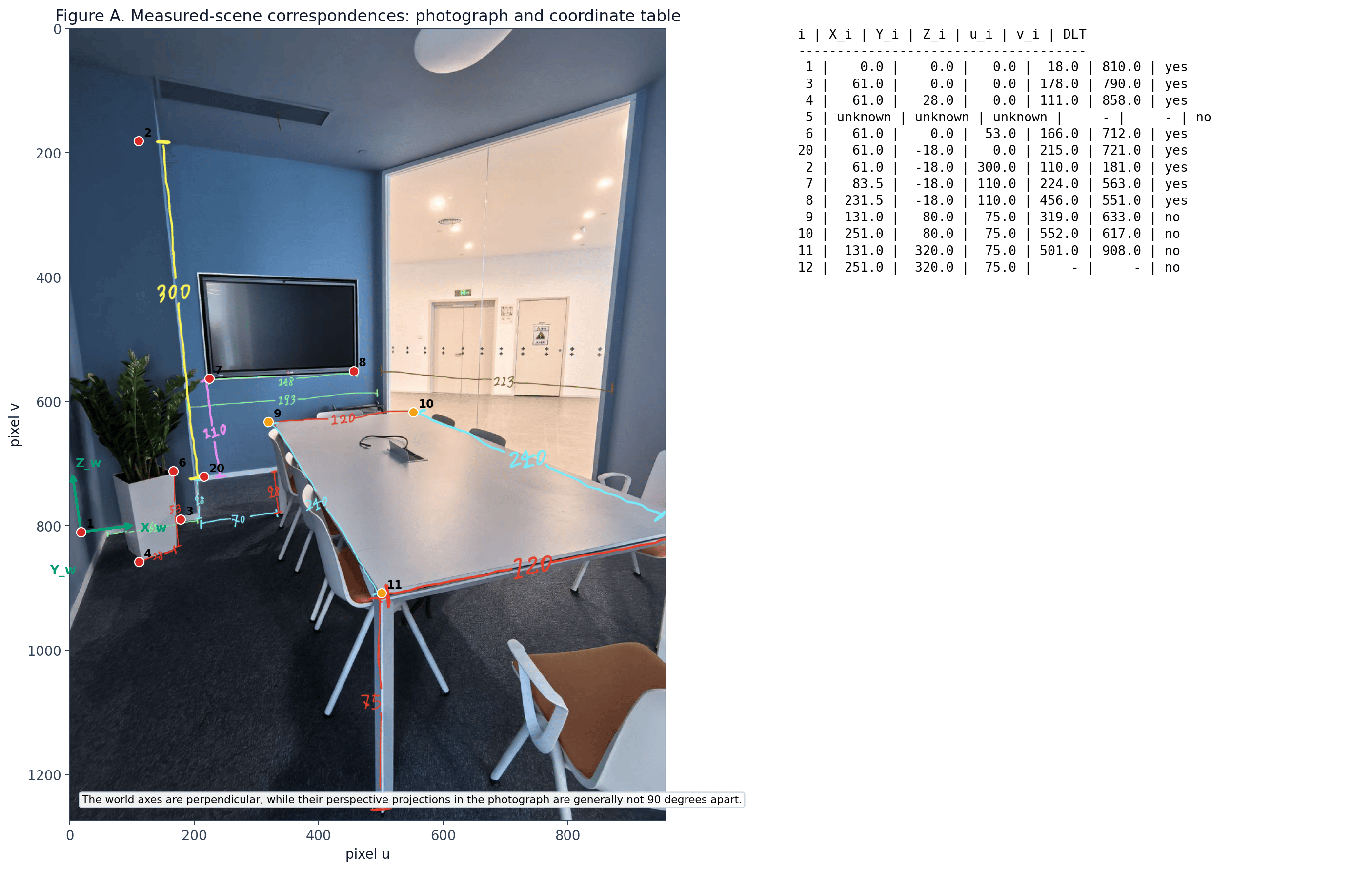
This experiment, by the section's author, mirrors the book's office example ([Figures 39.15](https://visionbook.mit.edu/imaging_geometry.html#fig-office_measurements) to [39.17](https://visionbook.mit.edu/imaging_geometry.html#fig-result_toymodel_3dscene_and_estimated_camera)) with a different scene: a photograph of a meeting room, scene measurements taken by hand in centimeters, hand-picked 3D-to-2D correspondences, a normalized DLT camera estimate, reprojection checks, and views of the measured scene.
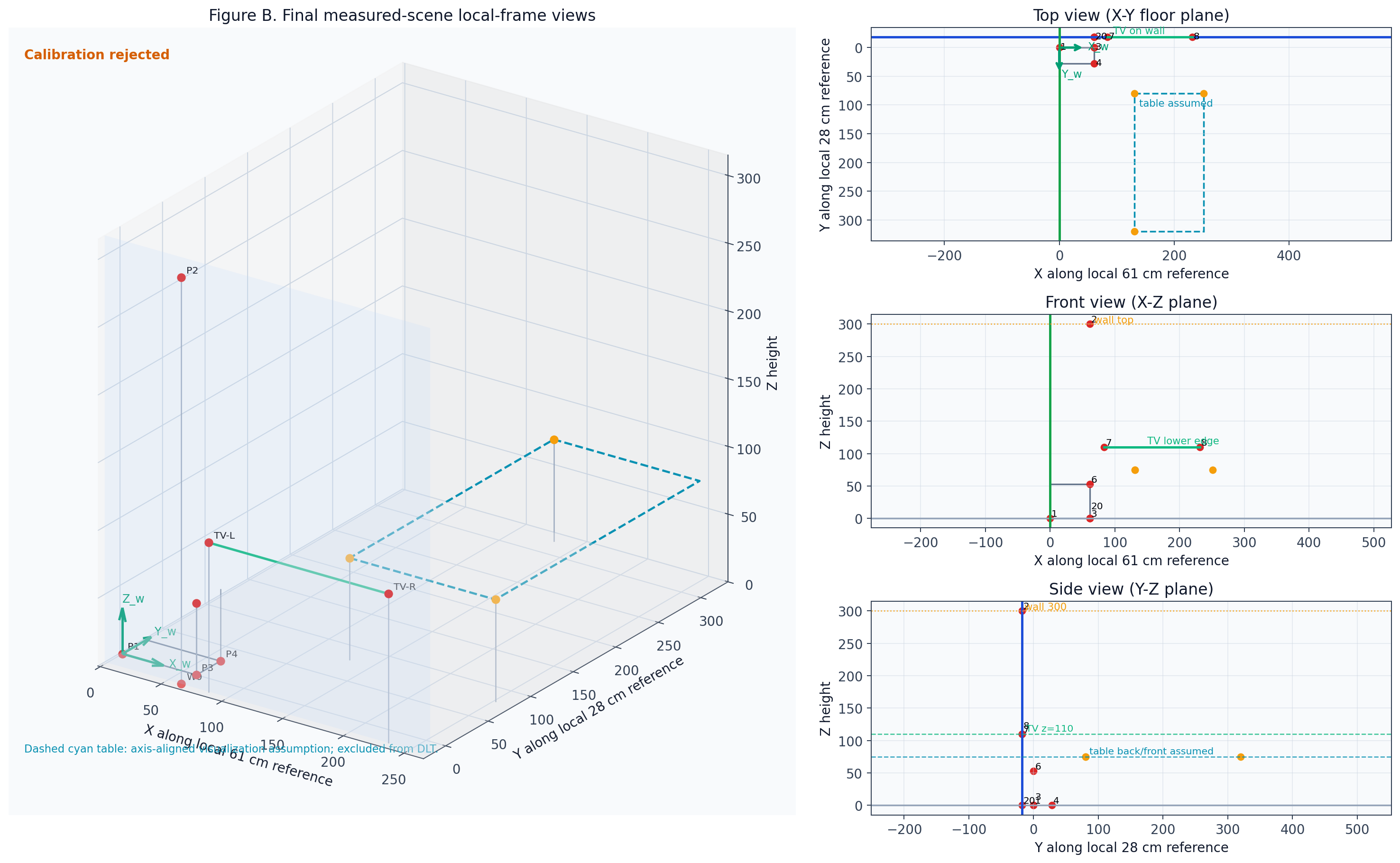
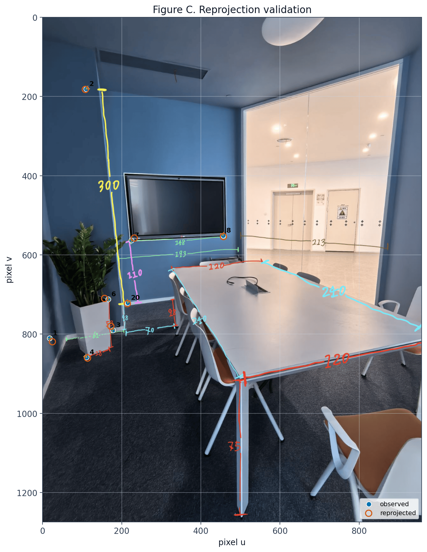
**The calibration fails, and that is the lesson.** The fitted camera reprojects the eight retained points with an RMS error of under 8 pixels, which looks good. But the recovered camera sits in an implausible place and looks away from the scene, and leaving out a single point moves the prediction by up to about 250 pixels. A low reprojection error on a handful of hand-measured points does not guarantee a physically correct camera. Real calibration needs many well-spread, non-coplanar correspondences, which is why practical methods use a calibration target seen from many views.
The measurements use a **local floor reference frame** next to the planter, not a full architectural room model. The origin `P1` is the left end of the green `61 cm` floor annotation, immediately to the left of the planter. From that point:
* `+X` follows the green `61 cm` floor segment from `P1` toward `P3`;
* `+Y` follows the red `28 cm` floor segment from `P3` toward `P4`;
* `+Z` points vertically upward.
So the floor is `Z = 0`. The blue television wall is modeled as the plane `Y = -18 cm`, because the cyan `18 cm` floor offset places the wall reference behind `P3`. The world axes are mutually perpendicular, while their perspective projections in the photograph are generally not 90 degrees apart. The code for this experiment is long and mostly bookkeeping, so only its printed diagnostics and figures are shown.
```output theme={null}
World coordinate convention for the measured scene:
- P1 = local planter-side floor reference, not a proven architectural room corner
- +X follows the 61 cm floor segment from P1 to P3
- +Y follows the 28 cm floor segment from P3 to P4
- +Z is vertically upward
- floor: Z = 0
- idealized blue-wall plane: Y = -18 cm
- W0 is the physical wall-floor reference at the bottom of the yellow 300 cm segment
- P2 is directly above W0, not above P3
- TV points lie on Y = -18 cm
- Table dimensions are measured, but table yaw relative to the local axes was not independently measured
Measurement table used for the final audited measured-scene model (centimeters):
```
```python theme={null}
print("Estimated projection matrix (normalized):")
print(M_est)
print(f"Mean reprojection error: {reproj_error.mean().item():.3f} px")
```
```output theme={null}
Estimated projection matrix (normalized):
tensor([[ 5.9194e-01, -7.8249e-02, 3.4478e-01, -7.8726e-02],
[-4.3553e-02, 5.6133e-01, 3.2921e-01, -3.0505e-01],
[-1.3287e-04, -1.7602e-04, 7.8526e-04, 3.0855e-04]],
dtype=torch.float64)
Mean reprojection error: 0.248 px
```
**Computational reconstruction related to Figure 39.14 of the book.**
The code generates synthetic 3D points, projects them with a known camera, adds small image noise, builds the DLT linear system, and estimates a projection matrix up to scale. The left panel compares observed and predicted image points, the center panel shows the stacked DLT system, and the right panel summarizes reprojection error.
### A real calibration attempt: a measured meeting room
This experiment, by the section's author, mirrors the book's office example ([Figures 39.15](https://visionbook.mit.edu/imaging_geometry.html#fig-office_measurements) to [39.17](https://visionbook.mit.edu/imaging_geometry.html#fig-result_toymodel_3dscene_and_estimated_camera)) with a different scene: a photograph of a meeting room, scene measurements taken by hand in centimeters, hand-picked 3D-to-2D correspondences, a normalized DLT camera estimate, reprojection checks, and views of the measured scene.
**The calibration fails, and that is the lesson.** The fitted camera reprojects the eight retained points with an RMS error of under 8 pixels, which looks good. But the recovered camera sits in an implausible place and looks away from the scene, and leaving out a single point moves the prediction by up to about 250 pixels. A low reprojection error on a handful of hand-measured points does not guarantee a physically correct camera. Real calibration needs many well-spread, non-coplanar correspondences, which is why practical methods use a calibration target seen from many views.
The measurements use a **local floor reference frame** next to the planter, not a full architectural room model. The origin `P1` is the left end of the green `61 cm` floor annotation, immediately to the left of the planter. From that point:
* `+X` follows the green `61 cm` floor segment from `P1` toward `P3`;
* `+Y` follows the red `28 cm` floor segment from `P3` toward `P4`;
* `+Z` points vertically upward.
So the floor is `Z = 0`. The blue television wall is modeled as the plane `Y = -18 cm`, because the cyan `18 cm` floor offset places the wall reference behind `P3`. The world axes are mutually perpendicular, while their perspective projections in the photograph are generally not 90 degrees apart. The code for this experiment is long and mostly bookkeeping, so only its printed diagnostics and figures are shown.
```output theme={null}
World coordinate convention for the measured scene:
- P1 = local planter-side floor reference, not a proven architectural room corner
- +X follows the 61 cm floor segment from P1 to P3
- +Y follows the 28 cm floor segment from P3 to P4
- +Z is vertically upward
- floor: Z = 0
- idealized blue-wall plane: Y = -18 cm
- W0 is the physical wall-floor reference at the bottom of the yellow 300 cm segment
- P2 is directly above W0, not above P3
- TV points lie on Y = -18 cm
- Table dimensions are measured, but table yaw relative to the local axes was not independently measured
Measurement table used for the final audited measured-scene model (centimeters):
```
| measurement | value\_cm | source segment | status |
|---|---|---|---|
| Local X reference P1 -> P3 | 61.00 | Green 61 cm floor annotation | direct |
| Local Y reference P3 -> P4 | 28.00 | Red 28 cm floor annotation | direct |
| Local Z reference P3 -> P6 | 53.00 | Red 53 cm vertical planter annotation | direct |
| Wall offset from P3 to W0 | 18.00 | Cyan 18 cm floor offset | direct |
| Wall height from W0 to P2 | 300.00 | Yellow 300 cm wall annotation | direct |
| TV wall span beginning at X=61 on Y=-18 | 193.00 | Green 193 cm annotation | direct |
| TV width along X | 148.00 | Green 148 cm annotation along the TV lower edge | direct |
| TV lower-left X coordinate | 83.50 | Derived as 61.0 + 22.5 | derived |
| TV lower-right X coordinate | 231.50 | Derived as 83.5 + 148.0 | derived |
| Table left X visualization coordinate | 131.00 | Derived as 61.0 + 70.0 | derived visualization assumption |
| Table back Y visualization coordinate | 80.00 | Derived as -18.0 + 98.0 | derived visualization assumption |
| Table width along X | 120.00 | Red 120 cm annotation | direct |
| Table length along Y | 240.00 | Cyan 240 cm annotation | direct |
| Table height along Z | 75.00 | Red 75 cm annotation | direct |
| id | feature | world coordinate | image coordinate | measurement endpoints | coordinate derivation | calibration use | status | exclusion reason |
|---|---|---|---|---|---|---|---|---|
| 1 | local floor origin | (np.float64(0.0), np.float64(0.0), np.float64(0.0)) | (np.float64(18.0), np.float64(810.0)) | left endpoint of green 61 cm segment | chosen local reference | used by DLT | manually selected from physical endpoint | - |
| 3 | end of 61 cm X segment | (np.float64(61.0), np.float64(0.0), np.float64(0.0)) | (np.float64(178.0), np.float64(790.0)) | green 61 cm segment | P1 + (61,0,0) | used by DLT | manually selected from physical endpoint | - |
| 4 | end of 28 cm Y segment | (np.float64(61.0), np.float64(28.0), np.float64(0.0)) | (np.float64(111.0), np.float64(858.0)) | red 28 cm segment from P3 to P4 | P3 + (0,28,0) | used by DLT | manually selected from physical endpoint | - |
| 5 | occluded planter upper-left corner | unknown | unavailable | vertical above P3-side planter corner | unknown because the physical corner is occluded | excluded from DLT | excluded | physical corner is occluded or ambiguous |
| 6 | top of 53 cm planter vertical | (np.float64(61.0), np.float64(0.0), np.float64(53.0)) | (np.float64(166.0), np.float64(712.0)) | red 53 cm segment from P3 to P6 | P3 + (0,0,53) | used by DLT | manually selected from physical endpoint | - |
| 20 | wall-floor reference at bottom of 300 cm segment | (np.float64(61.0), np.float64(-18.0), np.float64(0.0)) | (np.float64(215.0), np.float64(721.0)) | cyan 18 cm offset and yellow 300 cm bottom endpoint | P3 + (0,-18,0) | used by DLT | manually selected from physical endpoint | - |
| 2 | top of 300 cm wall reference | (np.float64(61.0), np.float64(-18.0), np.float64(300.0)) | (np.float64(110.0), np.float64(181.0)) | yellow 300 cm segment top endpoint | W0 + (0,0,300) | used by DLT | manually selected from physical endpoint; derived world coordinate | - |
| 7 | TV lower-left | (np.float64(83.5), np.float64(-18.0), np.float64(110.0)) | (np.float64(224.0), np.float64(563.0)) | centered 148 cm width inside 193 cm span on wall plane | derived world coordinate on Y=-18 plane | used by DLT | mechanically valid derived world coordinate; pixel manually selected | - |
| 8 | TV lower-right | (np.float64(231.5), np.float64(-18.0), np.float64(110.0)) | (np.float64(456.0), np.float64(551.0)) | centered 148 cm width inside 193 cm span on wall plane | derived world coordinate on Y=-18 plane | used by DLT | mechanically valid derived world coordinate; pixel manually selected | - |
| 9 | table back-left visualization point | (np.float64(131.0), np.float64(80.0), np.float64(75.0)) | (np.float64(319.0), np.float64(633.0)) | 61 cm reference, 70 cm X offset, 98 cm wall setback, 75 cm height | axis-aligned visualization assumption | excluded from DLT | excluded: orientation not measured | table yaw relative to local axes not independently measured |
| 10 | table back-right visualization point | (np.float64(251.0), np.float64(80.0), np.float64(75.0)) | (np.float64(552.0), np.float64(617.0)) | 120 cm table width | axis-aligned visualization assumption | excluded from DLT | excluded: orientation not measured | table yaw relative to local axes not independently measured |
| 11 | table front-left visualization point | (np.float64(131.0), np.float64(320.0), np.float64(75.0)) | (np.float64(501.0), np.float64(908.0)) | 240 cm table length | axis-aligned visualization assumption | excluded from DLT | excluded: orientation not measured | table yaw relative to local axes not independently measured |
| 12 | table front-right visualization point | (np.float64(251.0), np.float64(320.0), np.float64(75.0)) | unavailable | 120 cm width and 240 cm length | axis-aligned visualization assumption | excluded from DLT | excluded: endpoint ambiguous and orientation not measured | outside or not reliably visible |
 ```output theme={null}
Per-point reprojection summary:
```
```output theme={null}
Per-point reprojection summary:
```
| id | observed (u\_i, v\_i) | predicted (u\_i, v\_i) | fit error (px) | leave-one-out error (px) |
|---|---|---|---|---|
| 1 | (18.0, 810.0) | (24.7, 819.3) | 11.46 | 71.32 |
| 3 | (178.0, 790.0) | (172.5, 780.0) | 11.37 | 16.96 |
| 4 | (111.0, 858.0) | (113.6, 860.5) | 3.61 | 186.80 |
| 6 | (166.0, 712.0) | (156.5, 709.9) | 9.75 | 11.84 |
| 20 | (215.0, 721.0) | (214.2, 723.1) | 2.29 | 9.85 |
| 2 | (110.0, 181.0) | (108.0, 182.2) | 2.35 | 246.95 |
| 7 | (224.0, 563.0) | (231.7, 557.6) | 9.40 | 28.76 |
| 8 | (456.0, 551.0) | (457.0, 553.8) | 2.93 | 126.87 |