> ## Documentation Index
> Fetch the complete documentation index at: https://aegean.ai/llms.txt
> Use this file to discover all available pages before exploring further.
# Optimization and the ELBO
> Derivation of the Evidence Lower Bound from the KL divergence between the inference model and the true posterior, and why maximizing the ELBO jointly trains the encoder and decoder.
The [VAE architecture](/aiml-common/lectures/vae/vae-architecture/index) introduces an inference network $q(\mathbf z | \mathbf x ; \mathbf \phi)$ that approximates the intractable true posterior $p(\mathbf z | \mathbf x ; \mathbf \theta)$. Training jointly the encoder parameters $\mathbf \phi$ and the decoder parameters $\mathbf \theta$ requires an objective that is tractable yet aligned with maximizing the marginal log-likelihood $\log p(\mathbf x ; \mathbf \theta)$. The Evidence Lower Bound (ELBO) is exactly that objective.
## From KL divergence to the ELBO
During the treatment of entropy, we have met the concept of relative entropy or KL divergence that measures the "distance" between two distributions referenced on one of them.
$KL(q \,\|\, p) \;=\; \mathbb{E}_q\!\left[\log q(\mathbf x) - \log p(\mathbf x)\right] \;=\; -\sum_{\mathbf x} q(\mathbf x) \log \frac{p(\mathbf x)}{q(\mathbf x)}$
We will use KL divergence to obtain a suitable loss function that will be used in the optimization of this approximation via the $DNN_{enc}$ network. Ultimately we are trying to minimize the KL divergence between the true posterior $p(\mathbf z| \mathbf x ; \mathbf \theta)$ and the approximate posterior $q(\mathbf z | \mathbf x ; \mathbf \phi)$:
$KL(q(\mathbf z | \mathbf x ; \mathbf \phi) \,\|\, p(\mathbf z | \mathbf x; \mathbf \theta)) \;=\; -\sum_{\mathbf z} q(\mathbf z | \mathbf x ; \mathbf \phi) \log \frac{p(\mathbf z | \mathbf x; \mathbf \theta)}{q(\mathbf z | \mathbf x ; \mathbf \phi)}$
Applying Bayes' rule to replace the posterior $p(\mathbf z | \mathbf x; \mathbf \theta) = \frac{p(\mathbf z, \mathbf x; \mathbf \theta)}{p(\mathbf x; \mathbf \theta)}$:
$= -\sum_{\mathbf z} q(\mathbf z | \mathbf x ; \mathbf \phi) \log \frac{p(\mathbf z , \mathbf x; \mathbf \theta)}{q(\mathbf z | \mathbf x ; \mathbf \phi) \, p(\mathbf x; \mathbf \theta)}$
Separating the log of the product:
$= -\sum_{\mathbf z} q(\mathbf z | \mathbf x ; \mathbf \phi) \left[ \log \frac{p(\mathbf z , \mathbf x; \mathbf \theta)}{q(\mathbf z | \mathbf x ; \mathbf \phi)} - \log p(\mathbf x; \mathbf \theta) \right]$
Distributing the sum:
$= -\sum_{\mathbf z} q(\mathbf z | \mathbf x ; \mathbf \phi) \log \frac{p(\mathbf z , \mathbf x; \mathbf \theta)}{q(\mathbf z | \mathbf x ; \mathbf \phi)} + \sum_{\mathbf z} q(\mathbf z | \mathbf x ; \mathbf \phi) \log p(\mathbf x; \mathbf \theta)$
Since $\log p(\mathbf x; \mathbf \theta)$ does not depend on $\mathbf z$, it can be pulled out of the sum. And since $q$ is a valid distribution, $\sum_{\mathbf z} q(\mathbf z | \mathbf x ; \mathbf \phi) = 1$:
$= -\sum_{\mathbf z} q(\mathbf z | \mathbf x ; \mathbf \phi) \log \frac{p(\mathbf z , \mathbf x; \mathbf \theta)}{q(\mathbf z | \mathbf x ; \mathbf \phi)} + \log p(\mathbf x; \mathbf \theta)$
Rearranging:
$\Rightarrow \log p(\mathbf x; \mathbf \theta) \;=\; KL\!\left(q(\mathbf z | \mathbf x ; \mathbf \phi) \,\|\, p(\mathbf z | \mathbf x; \mathbf \theta)\right) \;+\; \underbrace{\sum_{\mathbf z} q(\mathbf z | \mathbf x ; \mathbf \phi) \log \frac{p(\mathbf z , \mathbf x; \mathbf \theta)}{q(\mathbf z | \mathbf x ; \mathbf \phi)}}_{\mathcal L(\phi, \theta) \,=\, \text{Evidence Lower Bound (ELBO)}}$
The bracketed quantity $\mathcal L(\phi, \theta)$ is the **Evidence Lower Bound (ELBO)**. It is a function of both the encoder parameters $\phi$ (through $q_\phi$) and the decoder parameters $\theta$ (through the joint $p_\theta(\mathbf z, \mathbf x)$).
## Why is it a lower bound?
The KL divergence is non-negative,
$KL\!\left(q(\mathbf z | \mathbf x ; \mathbf \phi) \,\|\, p(\mathbf z | \mathbf x; \mathbf \theta)\right) \;\ge\; 0,$
with equality if and only if $q(\mathbf z | \mathbf x ; \mathbf \phi) = p(\mathbf z | \mathbf x; \mathbf \theta)$ almost everywhere. Dropping the KL term from the equality above therefore turns it into an inequality:
$\log p(\mathbf x; \mathbf \theta) \;\ge\; \underbrace{\sum_{\mathbf z} q(\mathbf z | \mathbf x ; \mathbf \phi) \log \frac{p(\mathbf z , \mathbf x; \mathbf \theta)}{q(\mathbf z | \mathbf x ; \mathbf \phi)}}_{\mathcal L(\phi, \theta)}$
The KL is the **gap** between the bound and the true marginal log-likelihood. The closer the encoder approximates the true posterior, the tighter the bound.
## A practical form: reconstruction minus KL
The joint $p(\mathbf z, \mathbf x; \mathbf \theta)$ factors as $p(\mathbf x | \mathbf z ; \mathbf \theta)\, p(\mathbf z)$, where $p(\mathbf z)$ is the (fixed, parameter-free) prior — typically $\mathcal N(\mathbf 0, \mathbf I)$. Substituting and expanding the log:
$\mathcal L(\phi, \theta) \;=\; \underbrace{\mathbb{E}_{q_\phi(\mathbf z | \mathbf x)}\!\left[\log p(\mathbf x | \mathbf z; \mathbf \theta)\right]}_{\text{reconstruction term}} \;-\; \underbrace{KL\!\left(q_\phi(\mathbf z | \mathbf x) \,\|\, p(\mathbf z)\right)}_{\text{regularizer}}$
This is the form actually computed in code:
* The **reconstruction term** is the expected log-likelihood of the observed data $\mathbf x$ under the decoder when $\mathbf z$ is drawn from the encoder. Maximizing it pushes the decoder to put high probability on real data.
* The **KL regularizer** pulls the encoder's posterior toward the prior $p(\mathbf z)$. This prevents the encoder from collapsing into a different point distribution for every datapoint and is what makes the latent space dense and continuous.
Note carefully which KL is which: this regularizer uses the **prior** $p(\mathbf z)$, not the true posterior $p(\mathbf z | \mathbf x; \mathbf \theta)$. The KL against the true posterior is the (unobservable) bound gap from the previous section; the KL against the prior is part of the loss you actually optimize.
## Why is the ELBO useful for optimization?
Re-arrange the identity to put the ELBO on one side:
$\mathcal L(\phi, \theta) \;=\; \log p(\mathbf x; \mathbf \theta) \;-\; KL\!\left(q(\mathbf z | \mathbf x ; \mathbf \phi) \,\|\, p(\mathbf z | \mathbf x; \mathbf \theta)\right) \;\le\; \log p(\mathbf x; \mathbf \theta).$
Joint SGD over $(\phi, \theta)$ on the ELBO does two coupled jobs at once:
* **Encoder step (gradients on $\phi$).** With $\theta$ fixed, $\log p(\mathbf x; \mathbf \theta)$ is constant in $\phi$, so maximizing $\mathcal L$ over $\phi$ is *exactly* equivalent to minimizing the posterior KL. The encoder learns to track the true posterior, **tightening** the bound.
* **Decoder step (gradients on $\theta$).** The ELBO is a lower bound on $\log p(\mathbf x; \mathbf \theta)$, so increasing $\mathcal L$ over $\theta$ **raises** a lower bound on the marginal log-likelihood. The marginal itself rises only as fast as the bound is tight; the encoder's quality controls the slack.
The standard variational picture below illustrates this: the KL gap separates the ELBO from the true log-likelihood, and the gap closes only when $q_\phi$ matches the true posterior.
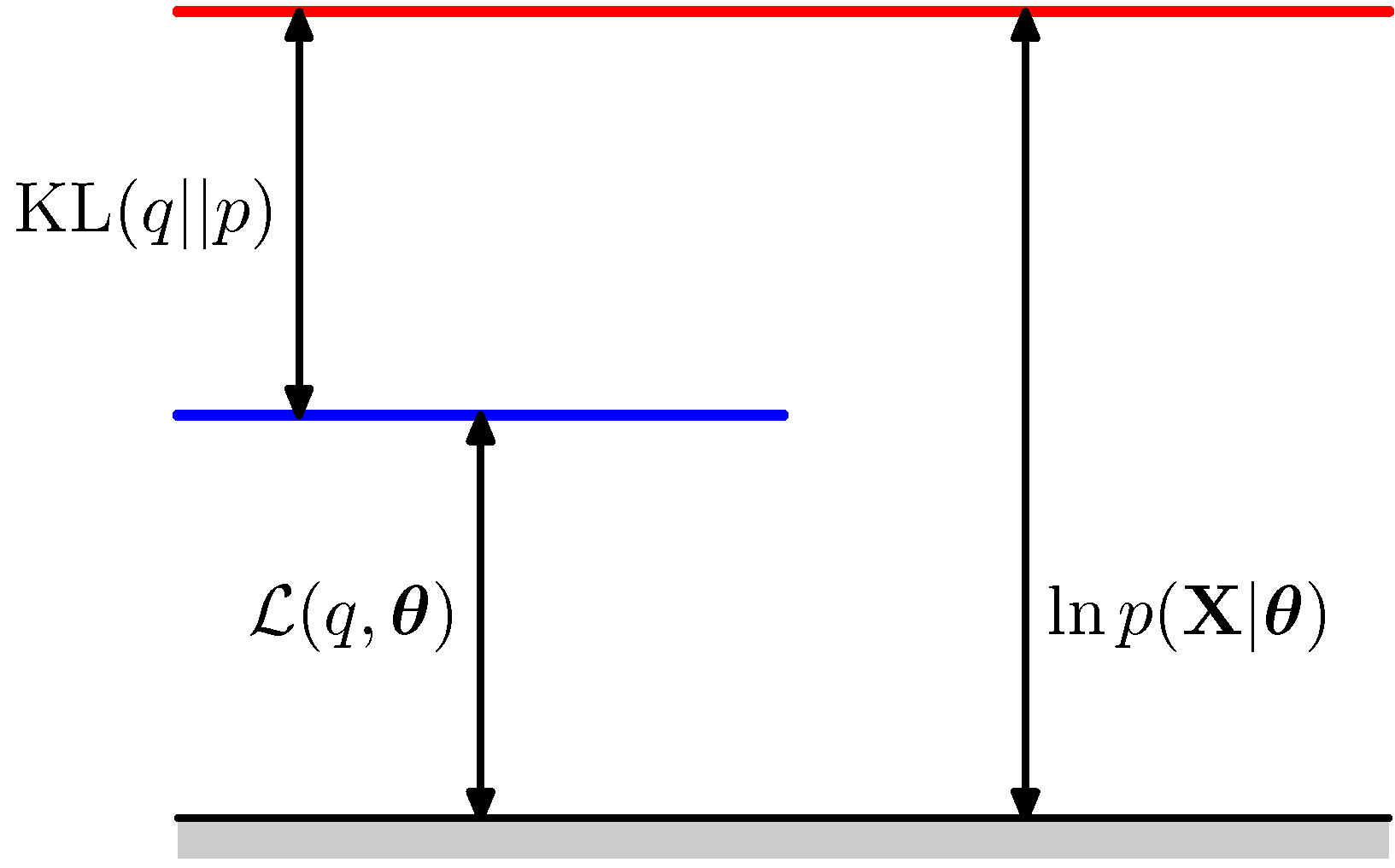 *KL represents the tightness of the ELBO bound*
In short: the ELBO is the surrogate that lets you train both networks with a single gradient. Optimizing it *better fits the data* (through $\theta$) and *better approximates the posterior* (through $\phi$) at the same time, with the second move keeping the first one honest.
This same ELBO reappears as the DDPM training loss when the single latent $\mathbf z$ is replaced by a Markov noise chain $\mathbf x_{1:T}$ and the encoder is fixed in advance — see [Training objective: from VAE ELBO to the DDPM loss](/aiml-common/lectures/diffusion/introduction/index#training-objective-from-vae-elbo-to-the-ddpm-loss) on the diffusion introduction page for the bridge.
***
[Edit this page on GitHub](https://github.com/aegean-ai/eaia/edit/main/src/aiml-common/lectures/vae/elbo-optimization/index.mdx) or [file an issue](https://github.com/aegean-ai/eaia/issues/new/choose).
*KL represents the tightness of the ELBO bound*
In short: the ELBO is the surrogate that lets you train both networks with a single gradient. Optimizing it *better fits the data* (through $\theta$) and *better approximates the posterior* (through $\phi$) at the same time, with the second move keeping the first one honest.
This same ELBO reappears as the DDPM training loss when the single latent $\mathbf z$ is replaced by a Markov noise chain $\mathbf x_{1:T}$ and the encoder is fixed in advance — see [Training objective: from VAE ELBO to the DDPM loss](/aiml-common/lectures/diffusion/introduction/index#training-objective-from-vae-elbo-to-the-ddpm-loss) on the diffusion introduction page for the bridge.
***
[Edit this page on GitHub](https://github.com/aegean-ai/eaia/edit/main/src/aiml-common/lectures/vae/elbo-optimization/index.mdx) or [file an issue](https://github.com/aegean-ai/eaia/issues/new/choose).