> ## Documentation Index
> Fetch the complete documentation index at: https://aegean.ai/llms.txt
> Use this file to discover all available pages before exploring further.
# VAE architecture
> Encoder-decoder architecture with variational inference and amortized posterior approximation.
In a previous section we have seen that VAE helps us define the latent space. The 'right' latent space is the one that makes the distribution $p(\mathbf z| \mathbf \theta)$ the most likely to produce $\mathbf x$. We are therefore introducing a stage that complements the aforementioned *generative model or decoder* given by $p(\mathbf x| \mathbf z ; \mathbf \theta) p(\mathbf z | \theta)$.
This stage is called the *recognition model or encoder* and is given by $p(\mathbf z| \mathbf x ; \mathbf \theta)$. The premise is this: the posterior $p(\mathbf z | \mathbf x ; \mathbf \theta)$ will result into a much more meaningful and compact latent space $\mathbf z$ than the prior $p(\mathbf z | \mathbf \theta)$. This encoding though, calls for sampling from a posterior that is itself intractable. We then need to use an approximation to such distribution: $q(\mathbf z| \mathbf x ; \mathbf \phi)$ and we call this the *inference model* that approximates the recognition model and help us optimize the marginal likelihood.
The VAE encoder-decoder spaces are shown below. The picture shows the more compact space that is defined by the encoder.
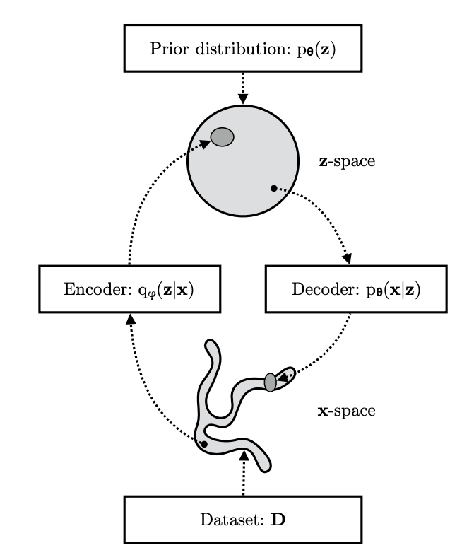 *VAE spaces and distributions (from [here](https://arxiv.org/pdf/1906.02691.pdf))*
The architecture of VAE includes four main components as shown below:
*VAE spaces and distributions (from [here](https://arxiv.org/pdf/1906.02691.pdf))*
The architecture of VAE includes four main components as shown below:
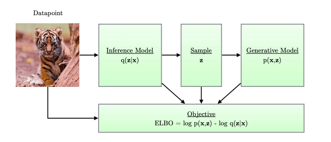 *VAE Architecture (from [here](https://arxiv.org/pdf/1906.02691.pdf))*
Similar to the generative model, the inference model can be, in general, a PGM of the form:
$q(\mathbf z | \mathbf x ; \mathbf \phi) = \prod_{j=1}^M q(\mathbf z_j | Pa(\mathbf z_j), \mathbf x ; \mathbf \phi)$
and this, similarly to the generative model, can be parametrized with a $DNN_{enc}(\phi)$. More specifically we obtain the approximation using the following construction:
$ (\mathbf \mu, \log \mathbf \Sigma ) = DNN_{enc}(\mathbf x, \mathbf \phi)$
$q(\mathbf z| \mathbf x ; \mathbf \phi) = N(\mathbf z; \mathbf \mu, \textsf{diag}(\mathbf \Sigma))$
The $DNN_{enc}$ implements amortized variational inference, that is, it estimates the posterior parameters over a batch of datapoints and this offers significant boost in the parameter learning.
With the encoder defined, the next question is how to train its parameters $\phi$ jointly with the decoder parameters $\theta$ when the true posterior $p(\mathbf z | \mathbf x; \mathbf \theta)$ is intractable. The answer is the **Evidence Lower Bound (ELBO)** — a tractable surrogate for the marginal log-likelihood that is derived from the KL divergence between $q$ and the true posterior. The derivation and its consequences for joint optimization are covered in the [Optimization and the ELBO](/aiml-common/lectures/vae/elbo-optimization/index) page.
## PyTorch reference
| PyTorch class | Description |
| -------------------------------------------------------------------------------- | ----------------------------------------------------------------------------- |
| [`nn.Linear`](https://docs.pytorch.org/docs/2.12/generated/torch.nn.Linear.html) | Applies an affine linear transformation to the incoming data: $y = xA^T + b$. |
***
[Edit this page on GitHub](https://github.com/aegean-ai/eaia/edit/main/src/aiml-common/lectures/vae/vae-architecture/index.mdx) or [file an issue](https://github.com/aegean-ai/eaia/issues/new/choose).
*VAE Architecture (from [here](https://arxiv.org/pdf/1906.02691.pdf))*
Similar to the generative model, the inference model can be, in general, a PGM of the form:
$q(\mathbf z | \mathbf x ; \mathbf \phi) = \prod_{j=1}^M q(\mathbf z_j | Pa(\mathbf z_j), \mathbf x ; \mathbf \phi)$
and this, similarly to the generative model, can be parametrized with a $DNN_{enc}(\phi)$. More specifically we obtain the approximation using the following construction:
$ (\mathbf \mu, \log \mathbf \Sigma ) = DNN_{enc}(\mathbf x, \mathbf \phi)$
$q(\mathbf z| \mathbf x ; \mathbf \phi) = N(\mathbf z; \mathbf \mu, \textsf{diag}(\mathbf \Sigma))$
The $DNN_{enc}$ implements amortized variational inference, that is, it estimates the posterior parameters over a batch of datapoints and this offers significant boost in the parameter learning.
With the encoder defined, the next question is how to train its parameters $\phi$ jointly with the decoder parameters $\theta$ when the true posterior $p(\mathbf z | \mathbf x; \mathbf \theta)$ is intractable. The answer is the **Evidence Lower Bound (ELBO)** — a tractable surrogate for the marginal log-likelihood that is derived from the KL divergence between $q$ and the true posterior. The derivation and its consequences for joint optimization are covered in the [Optimization and the ELBO](/aiml-common/lectures/vae/elbo-optimization/index) page.
## PyTorch reference
| PyTorch class | Description |
| -------------------------------------------------------------------------------- | ----------------------------------------------------------------------------- |
| [`nn.Linear`](https://docs.pytorch.org/docs/2.12/generated/torch.nn.Linear.html) | Applies an affine linear transformation to the incoming data: $y = xA^T + b$. |
***
[Edit this page on GitHub](https://github.com/aegean-ai/eaia/edit/main/src/aiml-common/lectures/vae/vae-architecture/index.mdx) or [file an issue](https://github.com/aegean-ai/eaia/issues/new/choose).