> ## Documentation Index
> Fetch the complete documentation index at: https://aegean.ai/llms.txt
> Use this file to discover all available pages before exploring further.
# Velocity fields
> Continuous-time vector fields that move particles through space, building from a storm analogy to the geometric foundation of flow matching and diffusion.
**Prerequisites.** If ODEs and the Euler integration step feel unfamiliar, work through [ODEs and the Euler method](/aiml-common/lectures/ml-math/calculus/odes-and-euler/index) first. The discrete update you write there is the same one used here to track particles through the storm field.
You already have an intuition for velocity fields, even if you have never seen the term. A storm has the same three properties:
* Wind has direction.
* Wind has magnitude.
* Different locations experience different winds.
A storm is, mathematically, a velocity field:
$$
\mathbf{v}(x, y, t)
$$
where the vector at each location $(x, y)$ at time $t$ tells you which way the air is moving and how fast.
## A rotating storm
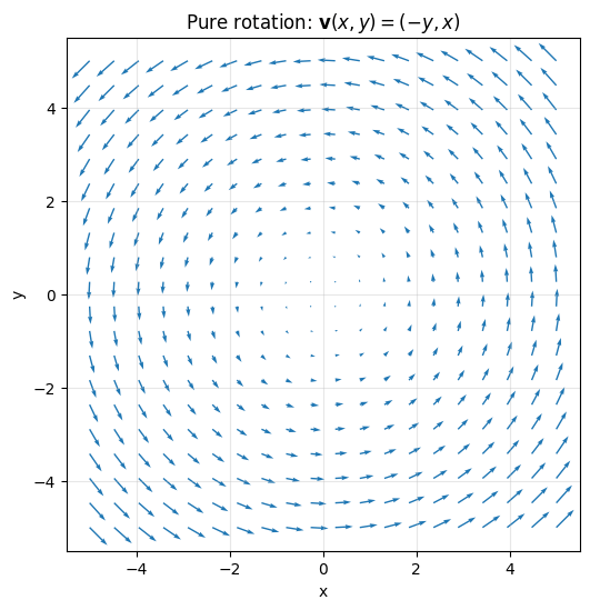
A simple 2D rotating storm centered at the origin is
$$
\mathbf{v}(x, y) =
\begin{bmatrix} -y \\ x \end{bmatrix}.
$$
This is a pure rotation. Two points pin down the picture:
* At $(1, 0)$: $\mathbf{v} = (0, 1)$, the wind blows upward.
* At $(0, 1)$: $\mathbf{v} = (-1, 0)$, the wind blows to the left.
So the field rotates counterclockwise around the origin.
```python theme={null}
import numpy as np
import matplotlib.pyplot as plt
x = np.linspace(-5, 5, 20)
y = np.linspace(-5, 5, 20)
X, Y = np.meshgrid(x, y)
U = -Y
V = X
fig, ax = plt.subplots(figsize=(6, 6))
ax.quiver(X, Y, U, V, color="C0")
ax.set_title("Pure rotation: $\\mathbf{v}(x, y) = (-y, x)$")
ax.set_xlabel("x"); ax.set_ylabel("y")
ax.set_aspect("equal")
ax.grid(alpha=0.3)
plt.show()
```
 ## Velocity weakens with distance
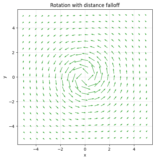
A real storm is strongest near the eye and weakens outward. A better model is
$$
\mathbf{v}(x, y) =
\frac{1}{x^2 + y^2 + \varepsilon}
\begin{bmatrix} -y \\ x \end{bmatrix},
$$
where $\varepsilon > 0$ avoids the singularity at the origin. Near the center the field is strong; far from the center it decays. The same plotting machinery shows the new structure.
```python theme={null}
eps = 0.5
norm = X**2 + Y**2 + eps
U = -Y / norm
V = X / norm
fig, ax = plt.subplots(figsize=(6, 6))
ax.quiver(X, Y, U, V, color="C2")
ax.set_title("Rotation with distance falloff")
ax.set_xlabel("x"); ax.set_ylabel("y")
ax.set_aspect("equal")
ax.grid(alpha=0.3)
plt.show()
```
## Velocity weakens with distance
A real storm is strongest near the eye and weakens outward. A better model is
$$
\mathbf{v}(x, y) =
\frac{1}{x^2 + y^2 + \varepsilon}
\begin{bmatrix} -y \\ x \end{bmatrix},
$$
where $\varepsilon > 0$ avoids the singularity at the origin. Near the center the field is strong; far from the center it decays. The same plotting machinery shows the new structure.
```python theme={null}
eps = 0.5
norm = X**2 + Y**2 + eps
U = -Y / norm
V = X / norm
fig, ax = plt.subplots(figsize=(6, 6))
ax.quiver(X, Y, U, V, color="C2")
ax.set_title("Rotation with distance falloff")
ax.set_xlabel("x"); ax.set_ylabel("y")
ax.set_aspect("equal")
ax.grid(alpha=0.3)
plt.show()
```
 ## Particles in the storm
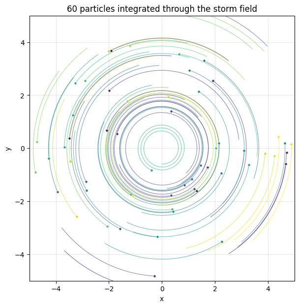
A velocity field becomes a dynamical system the moment you drop a particle in it. A particle at position $\mathbf{x}(t)$ moves according to
$$
\frac{d \mathbf{x}}{d t} = \mathbf{v}(\mathbf{x}).
$$
You can integrate this numerically. The simplest scheme is the Euler step,
$$
\mathbf{x}(t + \Delta t) = \mathbf{x}(t) + \Delta t \cdot \mathbf{v}(\mathbf{x}(t)),
$$
iterated for many steps. Release many particles at $t = 0$ and follow them: this is what raindrops, leaves, and debris do in a storm.
```python theme={null}
def storm_v(p, eps=0.5):
x, y = p[..., 0], p[..., 1]
norm = x**2 + y**2 + eps
return np.stack([-y / norm, x / norm], axis=-1)
rng = np.random.default_rng(0)
n_particles = 60
n_steps = 400
dt = 0.05
particles = rng.uniform(-4, 4, size=(n_particles, 2))
trajectories = np.empty((n_steps + 1, n_particles, 2))
trajectories[0] = particles
for step in range(n_steps):
trajectories[step + 1] = trajectories[step] + dt * storm_v(trajectories[step])
```
```python theme={null}
fig, ax = plt.subplots(figsize=(7, 7))
colors = plt.cm.viridis(np.linspace(0, 1, n_particles))
for i in range(n_particles):
ax.plot(trajectories[:, i, 0], trajectories[:, i, 1],
color=colors[i], alpha=0.6, lw=0.8)
ax.scatter(trajectories[-1, i, 0], trajectories[-1, i, 1],
color=colors[i], s=14, zorder=3, edgecolor="white", linewidth=0.5)
ax.set_title(f"{n_particles} particles integrated through the storm field")
ax.set_xlabel("x"); ax.set_ylabel("y")
ax.set_xlim(-5, 5); ax.set_ylim(-5, 5)
ax.set_aspect("equal")
ax.grid(alpha=0.3)
plt.show()
```
## Particles in the storm
A velocity field becomes a dynamical system the moment you drop a particle in it. A particle at position $\mathbf{x}(t)$ moves according to
$$
\frac{d \mathbf{x}}{d t} = \mathbf{v}(\mathbf{x}).
$$
You can integrate this numerically. The simplest scheme is the Euler step,
$$
\mathbf{x}(t + \Delta t) = \mathbf{x}(t) + \Delta t \cdot \mathbf{v}(\mathbf{x}(t)),
$$
iterated for many steps. Release many particles at $t = 0$ and follow them: this is what raindrops, leaves, and debris do in a storm.
```python theme={null}
def storm_v(p, eps=0.5):
x, y = p[..., 0], p[..., 1]
norm = x**2 + y**2 + eps
return np.stack([-y / norm, x / norm], axis=-1)
rng = np.random.default_rng(0)
n_particles = 60
n_steps = 400
dt = 0.05
particles = rng.uniform(-4, 4, size=(n_particles, 2))
trajectories = np.empty((n_steps + 1, n_particles, 2))
trajectories[0] = particles
for step in range(n_steps):
trajectories[step + 1] = trajectories[step] + dt * storm_v(trajectories[step])
```
```python theme={null}
fig, ax = plt.subplots(figsize=(7, 7))
colors = plt.cm.viridis(np.linspace(0, 1, n_particles))
for i in range(n_particles):
ax.plot(trajectories[:, i, 0], trajectories[:, i, 1],
color=colors[i], alpha=0.6, lw=0.8)
ax.scatter(trajectories[-1, i, 0], trajectories[-1, i, 1],
color=colors[i], s=14, zorder=3, edgecolor="white", linewidth=0.5)
ax.set_title(f"{n_particles} particles integrated through the storm field")
ax.set_xlabel("x"); ax.set_ylabel("y")
ax.set_xlim(-5, 5); ax.set_ylim(-5, 5)
ax.set_aspect("equal")
ax.grid(alpha=0.3)
plt.show()
```
 ***
[Edit this page on GitHub](https://github.com/aegean-ai/eaia/edit/main/src/aiml-common/lectures/velocity-fields/index.mdx) or [file an issue](https://github.com/aegean-ai/eaia/issues/new/choose).
***
[Edit this page on GitHub](https://github.com/aegean-ai/eaia/edit/main/src/aiml-common/lectures/velocity-fields/index.mdx) or [file an issue](https://github.com/aegean-ai/eaia/issues/new/choose).