> ## Documentation Index
> Fetch the complete documentation index at: https://aegean.ai/llms.txt
> Use this file to discover all available pages before exploring further.
# Learning Representations from Pixels
> Autoencoders, k-means, and contrastive learning on a toy colored-shapes dataset, where the chosen augmentation decides whether the embedding keeps shape or color.
 *This section was written by [Kaushik Kachireddy](https://github.com/kaushik0x7d2) ([pull request #82](https://github.com/pantelis/eng-ai-agents/pull/82)), with help from an AI coding agent (Claude Code) on the code. It reproduces the ideas of Chapter 30 of [*Foundations of Computer Vision*](https://visionbook.mit.edu/representation_learning.html) by Antonio Torralba, Phillip Isola, and William T. Freeman.*
**Representation learning** is the forward half of vision: mapping raw pixels to a compact **embedding** that exposes the underlying factors of a scene. This section builds the book's demonstrations on its toy **colored-shapes** dataset:
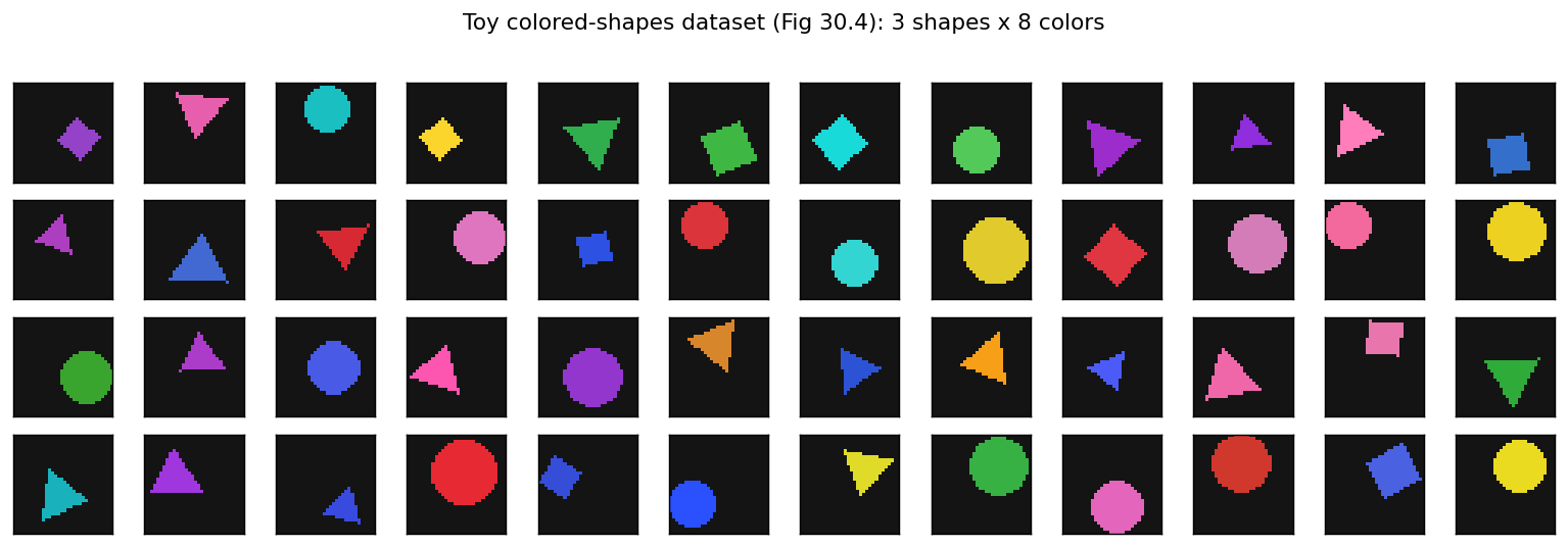
1. **The dataset** (Figure 30.4): 3 shapes by 8 colors, with random size, position, and rotation.
2. **Autoencoders** (Figure 30.5): an encoder, a bottleneck, and a decoder. You inspect the embedding through reconstructions, nearest neighbors, and a per-layer probe.
3. **K-means** (Figure 30.11): clustering as a discrete representation.
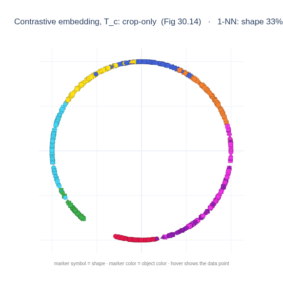
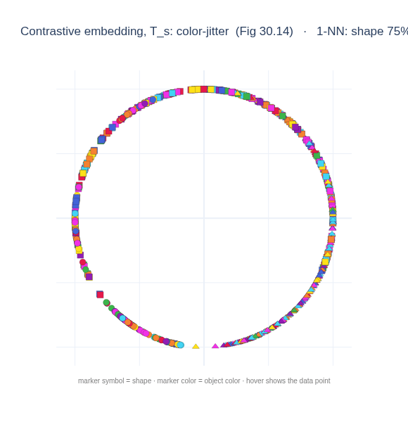
4. **Contrastive learning** (Figure 30.14): InfoNCE, where the choice of **data augmentation** decides whether the embedding encodes **color** or **shape**.
The colored-shapes data is procedural in the book too, so it is generated here exactly rather than loaded. Contrastive learning is also the idea behind [CLIP](/aiml-common/lectures/vlm/clip/index), the next section, which applies it across images and text.
```python theme={null}
import numpy as np, torch, torch.nn as nn, torch.nn.functional as F
import matplotlib.pyplot as plt
import plotly.io as pio
import importlib.util, shutil
if shutil.which('google-chrome') and importlib.util.find_spec('kaleido'): # a static PNG copy needs kaleido + Chrome
pio.renderers.default = 'plotly_mimetype+png' # interactive where supported, plus a static PNG
from PIL import Image, ImageDraw
device = 'cuda' if torch.cuda.is_available() else 'cpu'
_ = torch.manual_seed(0); np.random.seed(0)
torch.set_num_threads(max(1, torch.get_num_threads()))
plt.rcParams.update({'figure.dpi': 130, 'savefig.dpi': 130, 'image.interpolation': 'nearest', 'axes.grid': False})
print('device:', device)
# ---- the toy colored-shapes dataset (Figure 30.4 of the book) ----
COLORS = {'red':(220,50,50),'orange':(240,150,30),'yellow':(235,220,40),'green':(60,180,75),
'cyan':(40,200,200),'blue':(60,90,220),'purple':(150,60,200),'pink':(240,110,180)}
CNAMES = list(COLORS); SHAPES = ['circle','square','triangle']
def _one(rng, S=32):
ci, si = rng.integers(8), rng.integers(3)
base = np.array(COLORS[CNAMES[ci]], float)
col = tuple(int(np.clip(c + rng.normal(0, 12), 0, 255)) for c in base) # small color jitter
img = Image.new('RGB', (S, S), (20, 20, 20)); d = ImageDraw.Draw(img)
r = rng.integers(int(S*0.22), int(S*0.36)) # random size
cx, cy = rng.integers(r, S-r), rng.integers(r, S-r) # random position
ang = rng.uniform(0, 360) # random rotation
if si == 0:
d.ellipse([cx-r, cy-r, cx+r, cy+r], fill=col)
else:
n = 4 if si == 1 else 3
a0 = np.deg2rad(ang) + (np.pi/4 if si == 1 else -np.pi/2)
pts = [(cx+r*np.cos(a0+2*np.pi*k/n), cy+r*np.sin(a0+2*np.pi*k/n)) for k in range(n)]
d.polygon(pts, fill=col)
return np.asarray(img, np.float32)/255.0, si, ci
def make_dataset(n, seed, S=32):
rng = np.random.default_rng(seed)
X = np.zeros((n, S, S, 3), np.float32); ys = np.zeros(n, int); yc = np.zeros(n, int)
for i in range(n): X[i], ys[i], yc[i] = _one(rng, S)
return X, ys, yc
Xtr, ys_tr, yc_tr = make_dataset(3000, seed=0)
Xte, ys_te, yc_te = make_dataset(600, seed=99)
Xtr_t = torch.tensor(Xtr).permute(0, 3, 1, 2); Xte_t = torch.tensor(Xte).permute(0, 3, 1, 2)
print('train', Xtr.shape, ' test', Xte.shape)
```
```output theme={null}
device: cuda
```
```output theme={null}
train (3000, 32, 32, 3) test (600, 32, 32, 3)
```
## The colored-shapes dataset
Each image has one of **three shapes** (circle, square, triangle) in one of **eight colors**, with random size, position and rotation. Two independent factors, **shape** and **color**, which a representation to disentangle.
*This section was written by [Kaushik Kachireddy](https://github.com/kaushik0x7d2) ([pull request #82](https://github.com/pantelis/eng-ai-agents/pull/82)), with help from an AI coding agent (Claude Code) on the code. It reproduces the ideas of Chapter 30 of [*Foundations of Computer Vision*](https://visionbook.mit.edu/representation_learning.html) by Antonio Torralba, Phillip Isola, and William T. Freeman.*
**Representation learning** is the forward half of vision: mapping raw pixels to a compact **embedding** that exposes the underlying factors of a scene. This section builds the book's demonstrations on its toy **colored-shapes** dataset:
1. **The dataset** (Figure 30.4): 3 shapes by 8 colors, with random size, position, and rotation.
2. **Autoencoders** (Figure 30.5): an encoder, a bottleneck, and a decoder. You inspect the embedding through reconstructions, nearest neighbors, and a per-layer probe.
3. **K-means** (Figure 30.11): clustering as a discrete representation.
4. **Contrastive learning** (Figure 30.14): InfoNCE, where the choice of **data augmentation** decides whether the embedding encodes **color** or **shape**.
The colored-shapes data is procedural in the book too, so it is generated here exactly rather than loaded. Contrastive learning is also the idea behind [CLIP](/aiml-common/lectures/vlm/clip/index), the next section, which applies it across images and text.
```python theme={null}
import numpy as np, torch, torch.nn as nn, torch.nn.functional as F
import matplotlib.pyplot as plt
import plotly.io as pio
import importlib.util, shutil
if shutil.which('google-chrome') and importlib.util.find_spec('kaleido'): # a static PNG copy needs kaleido + Chrome
pio.renderers.default = 'plotly_mimetype+png' # interactive where supported, plus a static PNG
from PIL import Image, ImageDraw
device = 'cuda' if torch.cuda.is_available() else 'cpu'
_ = torch.manual_seed(0); np.random.seed(0)
torch.set_num_threads(max(1, torch.get_num_threads()))
plt.rcParams.update({'figure.dpi': 130, 'savefig.dpi': 130, 'image.interpolation': 'nearest', 'axes.grid': False})
print('device:', device)
# ---- the toy colored-shapes dataset (Figure 30.4 of the book) ----
COLORS = {'red':(220,50,50),'orange':(240,150,30),'yellow':(235,220,40),'green':(60,180,75),
'cyan':(40,200,200),'blue':(60,90,220),'purple':(150,60,200),'pink':(240,110,180)}
CNAMES = list(COLORS); SHAPES = ['circle','square','triangle']
def _one(rng, S=32):
ci, si = rng.integers(8), rng.integers(3)
base = np.array(COLORS[CNAMES[ci]], float)
col = tuple(int(np.clip(c + rng.normal(0, 12), 0, 255)) for c in base) # small color jitter
img = Image.new('RGB', (S, S), (20, 20, 20)); d = ImageDraw.Draw(img)
r = rng.integers(int(S*0.22), int(S*0.36)) # random size
cx, cy = rng.integers(r, S-r), rng.integers(r, S-r) # random position
ang = rng.uniform(0, 360) # random rotation
if si == 0:
d.ellipse([cx-r, cy-r, cx+r, cy+r], fill=col)
else:
n = 4 if si == 1 else 3
a0 = np.deg2rad(ang) + (np.pi/4 if si == 1 else -np.pi/2)
pts = [(cx+r*np.cos(a0+2*np.pi*k/n), cy+r*np.sin(a0+2*np.pi*k/n)) for k in range(n)]
d.polygon(pts, fill=col)
return np.asarray(img, np.float32)/255.0, si, ci
def make_dataset(n, seed, S=32):
rng = np.random.default_rng(seed)
X = np.zeros((n, S, S, 3), np.float32); ys = np.zeros(n, int); yc = np.zeros(n, int)
for i in range(n): X[i], ys[i], yc[i] = _one(rng, S)
return X, ys, yc
Xtr, ys_tr, yc_tr = make_dataset(3000, seed=0)
Xte, ys_te, yc_te = make_dataset(600, seed=99)
Xtr_t = torch.tensor(Xtr).permute(0, 3, 1, 2); Xte_t = torch.tensor(Xte).permute(0, 3, 1, 2)
print('train', Xtr.shape, ' test', Xte.shape)
```
```output theme={null}
device: cuda
```
```output theme={null}
train (3000, 32, 32, 3) test (600, 32, 32, 3)
```
## The colored-shapes dataset
Each image has one of **three shapes** (circle, square, triangle) in one of **eight colors**, with random size, position and rotation. Two independent factors, **shape** and **color**, which a representation to disentangle.
 ## Autoencoders
An **autoencoder** maps each image through a low-dimensional **bottleneck** and back, trained to reconstruct its input: $\min_{f,g}\;\mathbb{E}_x\,\lVert g(f(x))-x\rVert^2$. The bottleneck $f(x)$ is forced to keep only what is needed to redraw the image, so it becomes a compact **representation**. You train a small convolutional autoencoder and then look at what its embedding captures.
```python theme={null}
def cbr(i, o, s): return nn.Sequential(nn.Conv2d(i, o, 3, s, 1), nn.ReLU())
class AE(nn.Module):
'''The book's autoencoder: six conv layers + a 128-d bottleneck. Downsampling stops
at 4x4 so deep features keep the spatial detail that distinguishes the shapes.'''
def __init__(self, M=128):
super().__init__()
self.c = nn.ModuleList([cbr(3, 24, 2), cbr(24, 48, 1), cbr(48, 64, 2),
cbr(64, 96, 1), cbr(96, 128, 2), cbr(128, 128, 1)]) # 32->16->16->8->8->4->4
self.bott = nn.Linear(128 * 16, M)
self.dec = nn.Sequential(nn.Linear(M, 128 * 16), nn.ReLU(), nn.Unflatten(1, (128, 4, 4)),
nn.ConvTranspose2d(128, 64, 4, 2, 1), nn.ReLU(),
nn.ConvTranspose2d(64, 32, 4, 2, 1), nn.ReLU(),
nn.ConvTranspose2d(32, 3, 4, 2, 1), nn.Sigmoid())
def feats(self, x): # input + each of the 6 conv layers (for the probe)
outs = [x.flatten(1)]; h = x
for conv in self.c: h = conv(h); outs.append(h.flatten(1))
return outs
def encode(self, x):
h = x
for conv in self.c: h = conv(h)
return self.bott(h.flatten(1)) # the 128-d embedding
def forward(self, x):
z = self.encode(x); return self.dec(z), z
ae = AE().to(device); opt = torch.optim.Adam(ae.parameters(), 1e-3); lossf = nn.MSELoss()
N = len(Xtr_t)
# The Figure 30.5b crossing needs a real training budget (20k steps): a few minutes on a GPU.
AE_STEPS = 20000
for step in range(AE_STEPS):
xb = Xtr_t[torch.randint(0, N, (128,))].to(device)
out, _ = ae(xb); loss = lossf(out, xb)
opt.zero_grad(); loss.backward(); opt.step()
print(f'autoencoder ({AE_STEPS} steps) trained, reconstruction MSE {loss.item():.4f}')
```
```output theme={null}
autoencoder (20000 steps) trained, reconstruction MSE 0.0004
```
### Reconstructions and nearest neighbors
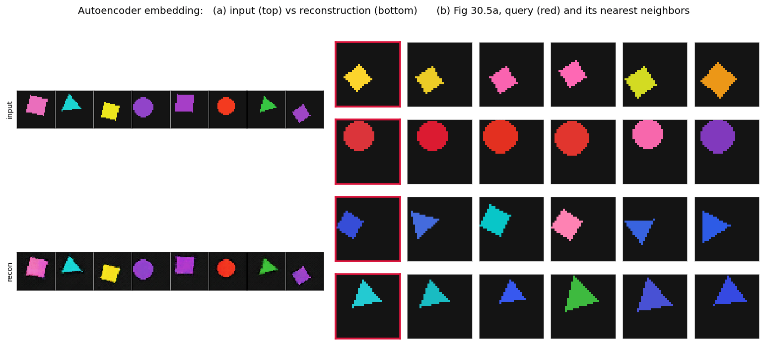
The reconstructions confirm the bottleneck preserves shape, color and rough pose. More interesting: images whose embeddings are **nearest neighbors** tend to share both shape and color: the embedding has organized the data by its true factors.
```python theme={null}
ae.eval()
with torch.no_grad():
recon, _ = ae(Xte_t[:8].to(device)); recon = recon.cpu()
Ztr = ae.encode(Xtr_t.to(device)).cpu()
Ztr = F.normalize(Ztr, dim=1)
```
## Autoencoders
An **autoencoder** maps each image through a low-dimensional **bottleneck** and back, trained to reconstruct its input: $\min_{f,g}\;\mathbb{E}_x\,\lVert g(f(x))-x\rVert^2$. The bottleneck $f(x)$ is forced to keep only what is needed to redraw the image, so it becomes a compact **representation**. You train a small convolutional autoencoder and then look at what its embedding captures.
```python theme={null}
def cbr(i, o, s): return nn.Sequential(nn.Conv2d(i, o, 3, s, 1), nn.ReLU())
class AE(nn.Module):
'''The book's autoencoder: six conv layers + a 128-d bottleneck. Downsampling stops
at 4x4 so deep features keep the spatial detail that distinguishes the shapes.'''
def __init__(self, M=128):
super().__init__()
self.c = nn.ModuleList([cbr(3, 24, 2), cbr(24, 48, 1), cbr(48, 64, 2),
cbr(64, 96, 1), cbr(96, 128, 2), cbr(128, 128, 1)]) # 32->16->16->8->8->4->4
self.bott = nn.Linear(128 * 16, M)
self.dec = nn.Sequential(nn.Linear(M, 128 * 16), nn.ReLU(), nn.Unflatten(1, (128, 4, 4)),
nn.ConvTranspose2d(128, 64, 4, 2, 1), nn.ReLU(),
nn.ConvTranspose2d(64, 32, 4, 2, 1), nn.ReLU(),
nn.ConvTranspose2d(32, 3, 4, 2, 1), nn.Sigmoid())
def feats(self, x): # input + each of the 6 conv layers (for the probe)
outs = [x.flatten(1)]; h = x
for conv in self.c: h = conv(h); outs.append(h.flatten(1))
return outs
def encode(self, x):
h = x
for conv in self.c: h = conv(h)
return self.bott(h.flatten(1)) # the 128-d embedding
def forward(self, x):
z = self.encode(x); return self.dec(z), z
ae = AE().to(device); opt = torch.optim.Adam(ae.parameters(), 1e-3); lossf = nn.MSELoss()
N = len(Xtr_t)
# The Figure 30.5b crossing needs a real training budget (20k steps): a few minutes on a GPU.
AE_STEPS = 20000
for step in range(AE_STEPS):
xb = Xtr_t[torch.randint(0, N, (128,))].to(device)
out, _ = ae(xb); loss = lossf(out, xb)
opt.zero_grad(); loss.backward(); opt.step()
print(f'autoencoder ({AE_STEPS} steps) trained, reconstruction MSE {loss.item():.4f}')
```
```output theme={null}
autoencoder (20000 steps) trained, reconstruction MSE 0.0004
```
### Reconstructions and nearest neighbors
The reconstructions confirm the bottleneck preserves shape, color and rough pose. More interesting: images whose embeddings are **nearest neighbors** tend to share both shape and color: the embedding has organized the data by its true factors.
```python theme={null}
ae.eval()
with torch.no_grad():
recon, _ = ae(Xte_t[:8].to(device)); recon = recon.cpu()
Ztr = ae.encode(Xtr_t.to(device)).cpu()
Ztr = F.normalize(Ztr, dim=1)
```
 ### What does each layer encode?
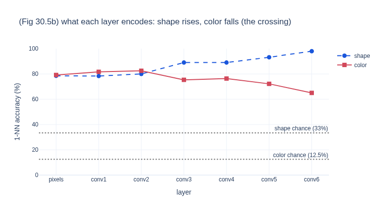
Probe every layer with a **1-nearest-neighbor classifier** (train features -> predict a test image's shape / color). The two factors are read out very differently across depth: **shape accuracy rises toward \~99%** in the deeper, more semantic features, while **color accuracy falls** as the network abstracts away low-level appearance: the **crossing** the book reports (Fig 30.5b). Reproducing it needs the book's architecture (six conv layers, keeping spatial detail) and a real training budget; a too-shallow model, or downsampling all the way to a single vector, does not show it.
```python theme={null}
def nn_acc(tr, te, ytr, yte):
tr = F.normalize(tr, dim=1); te = F.normalize(te, dim=1)
return (ytr[(te @ tr.T).argmax(1).numpy()] == yte).mean()
# Stream the probe layer-by-layer (forward train+test together, keep only the current
# activations) so we never hold all seven layers' features at once, memory-lean.
ae.eval(); layers = ['pixels', 'conv1', 'conv2', 'conv3', 'conv4', 'conv5', 'conv6']
acc_s, acc_c = [], []
with torch.no_grad():
htr, hte = Xtr_t.to(device), Xte_t.to(device)
for i, conv in enumerate([None] + list(ae.c)):
if conv is not None: htr = conv(htr); hte = conv(hte)
tr, te = htr.flatten(1).cpu(), hte.flatten(1).cpu()
acc_s.append(nn_acc(tr, te, ys_tr, ys_te) * 100)
acc_c.append(nn_acc(tr, te, yc_tr, yc_te) * 100)
del tr, te
```
### What does each layer encode?
Probe every layer with a **1-nearest-neighbor classifier** (train features -> predict a test image's shape / color). The two factors are read out very differently across depth: **shape accuracy rises toward \~99%** in the deeper, more semantic features, while **color accuracy falls** as the network abstracts away low-level appearance: the **crossing** the book reports (Fig 30.5b). Reproducing it needs the book's architecture (six conv layers, keeping spatial detail) and a real training budget; a too-shallow model, or downsampling all the way to a single vector, does not show it.
```python theme={null}
def nn_acc(tr, te, ytr, yte):
tr = F.normalize(tr, dim=1); te = F.normalize(te, dim=1)
return (ytr[(te @ tr.T).argmax(1).numpy()] == yte).mean()
# Stream the probe layer-by-layer (forward train+test together, keep only the current
# activations) so we never hold all seven layers' features at once, memory-lean.
ae.eval(); layers = ['pixels', 'conv1', 'conv2', 'conv3', 'conv4', 'conv5', 'conv6']
acc_s, acc_c = [], []
with torch.no_grad():
htr, hte = Xtr_t.to(device), Xte_t.to(device)
for i, conv in enumerate([None] + list(ae.c)):
if conv is not None: htr = conv(htr); hte = conv(hte)
tr, te = htr.flatten(1).cpu(), hte.flatten(1).cpu()
acc_s.append(nn_acc(tr, te, ys_tr, ys_te) * 100)
acc_c.append(nn_acc(tr, te, yc_tr, yc_te) * 100)
del tr, te
```
 ```output theme={null}
shape: ['78', '78', '80', '89', '89', '93', '98']
color: ['79', '82', '82', '75', '76', '72', '65']
```
## K-means clustering
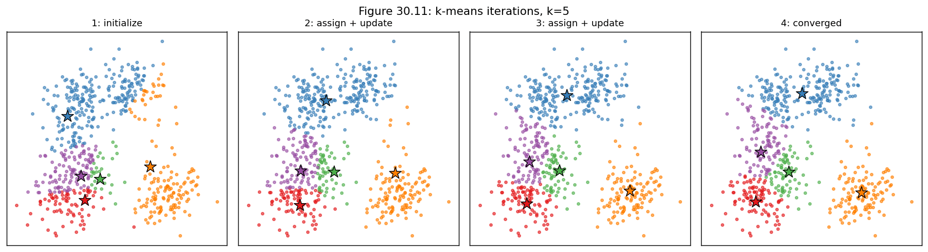
Clustering yields a **discrete** representation: each point is summarized by the index of its nearest code vector. **K-means** minimises $\sum_i \lVert z_{a_i} - x^{(i)}\rVert^2$ by block-coordinate descent, alternating:
**(assign)** each point to its nearest mean, **(update)** each mean to the average of its assigned points. The figure shows the first iterations on a 2-D dataset with $k=5$ (Fig 30.11).
```python theme={null}
g = np.random.default_rng(2)
centers_true = g.uniform(-1, 1, (5, 2)) * 2.2
pts = np.concatenate([c + g.normal(0, 0.45, (120, 2)) for c in centers_true])
k = 5
z = pts[g.choice(len(pts), k, replace=False)].copy() # init code vectors
palette = np.array(['#e41a1c', '#377eb8', '#4daf4a', '#984ea3', '#ff7f00'])
snaps = []
for it in range(4):
a = np.argmin(((pts[:, None, :] - z[None]) ** 2).sum(2), axis=1) # assign
snaps.append((z.copy(), a.copy()))
for j in range(k):
if (a == j).any(): z[j] = pts[a == j].mean(0) # update
```
```output theme={null}
shape: ['78', '78', '80', '89', '89', '93', '98']
color: ['79', '82', '82', '75', '76', '72', '65']
```
## K-means clustering
Clustering yields a **discrete** representation: each point is summarized by the index of its nearest code vector. **K-means** minimises $\sum_i \lVert z_{a_i} - x^{(i)}\rVert^2$ by block-coordinate descent, alternating:
**(assign)** each point to its nearest mean, **(update)** each mean to the average of its assigned points. The figure shows the first iterations on a 2-D dataset with $k=5$ (Fig 30.11).
```python theme={null}
g = np.random.default_rng(2)
centers_true = g.uniform(-1, 1, (5, 2)) * 2.2
pts = np.concatenate([c + g.normal(0, 0.45, (120, 2)) for c in centers_true])
k = 5
z = pts[g.choice(len(pts), k, replace=False)].copy() # init code vectors
palette = np.array(['#e41a1c', '#377eb8', '#4daf4a', '#984ea3', '#ff7f00'])
snaps = []
for it in range(4):
a = np.argmin(((pts[:, None, :] - z[None]) ** 2).sum(2), axis=1) # assign
snaps.append((z.copy(), a.copy()))
for j in range(k):
if (a == j).any(): z[j] = pts[a == j].mean(0) # update
```
 ## Contrastive learning: the augmentation chooses the invariance
**Contrastive learning** pulls together two augmented **views** of the same image (a *positive* pair) while pushing apart different images, via the **InfoNCE** loss:
$\mathcal{L} = -\log \frac{e^{f(x)^\top f(x^+)/\tau}}{e^{f(x)^\top f(x^+)/\tau} + \sum_i e^{f(x)^\top f(x_i^-)/\tau}}.$
The representation becomes **invariant** to whatever the augmentation changes. So the *choice of augmentation* decides which factor survives (embedding dimension $M=2$, so it can be plotted directly on the unit circle):
* **crop only** ($T_c$): keeps color, varies which part of the shape is seen -> the embedding organizes by **color**;
* **color jitter** ($T_s$): destroys color, keeps shape -> the embedding organizes by **shape**.
```python theme={null}
class Enc(nn.Module):
def __init__(self):
super().__init__()
self.net = nn.Sequential(nn.Conv2d(3, 16, 3, 2, 1), nn.ReLU(), nn.Conv2d(16, 32, 3, 2, 1), nn.ReLU(),
nn.Conv2d(32, 64, 3, 2, 1), nn.ReLU(), nn.Flatten(), nn.Linear(64*16, 64), nn.ReLU(), nn.Linear(64, 2))
def forward(self, x): return F.normalize(self.net(x), dim=1) # onto the unit circle
def rand_crop(xb, lo=0.5):
N, C, H, W = xb.shape; out = torch.empty_like(xb)
for i in range(N):
s = float(torch.empty(1).uniform_(lo, 1.0)); ch = max(8, int(H*s)); cw = max(8, int(W*s))
top = int(torch.randint(0, H-ch+1, (1,))); left = int(torch.randint(0, W-cw+1, (1,)))
out[i] = F.interpolate(xb[i:i+1, :, top:top+ch, left:left+cw], size=(H, W), mode='bilinear', align_corners=False)[0]
return out
def color_jitter(xb):
N = xb.shape[0]; gain = torch.empty(N, 3, 1, 1, device=xb.device).uniform_(0.4, 1.6)
bright = torch.empty(N, 1, 1, 1, device=xb.device).uniform_(0.6, 1.4)
perm = torch.stack([torch.randperm(3) for _ in range(N)])
xj = torch.stack([xb[i, perm[i]] for i in range(N)])
return (xj * gain * bright).clamp(0, 1)
def small_shift(xb):
sh = torch.randint(-3, 4, (2,)); return torch.roll(xb, (int(sh[0]), int(sh[1])), dims=(2, 3))
def infonce(z1, z2, tau=0.2):
z = torch.cat([z1, z2]); sim = z @ z.T / tau; n = len(z1)
sim.fill_diagonal_(-1e9)
targets = torch.cat([torch.arange(n) + n, torch.arange(n)]).to(z.device)
return F.cross_entropy(sim, targets)
def train_contrastive(aug, steps, bs=128, seed=1):
_ = torch.manual_seed(seed); net = Enc().to(device); opt = torch.optim.Adam(net.parameters(), 1e-3)
for st in range(steps):
xb = Xtr_t[torch.randint(0, N, (bs,))].to(device)
loss = infonce(net(aug(xb)), net(aug(xb))); opt.zero_grad(); loss.backward(); opt.step()
net.eval()
with torch.no_grad(): Z = net(Xtr_t.to(device)).cpu().numpy()
return Z
Z_color = train_contrastive(lambda x: rand_crop(x), steps=1500) # crop only -> color
Z_shape = train_contrastive(lambda x: color_jitter(small_shift(x)), steps=2500) # jitter -> shape
print('trained both contrastive encoders')
```
```output theme={null}
trained both contrastive encoders
```
## Contrastive learning: the augmentation chooses the invariance
**Contrastive learning** pulls together two augmented **views** of the same image (a *positive* pair) while pushing apart different images, via the **InfoNCE** loss:
$\mathcal{L} = -\log \frac{e^{f(x)^\top f(x^+)/\tau}}{e^{f(x)^\top f(x^+)/\tau} + \sum_i e^{f(x)^\top f(x_i^-)/\tau}}.$
The representation becomes **invariant** to whatever the augmentation changes. So the *choice of augmentation* decides which factor survives (embedding dimension $M=2$, so it can be plotted directly on the unit circle):
* **crop only** ($T_c$): keeps color, varies which part of the shape is seen -> the embedding organizes by **color**;
* **color jitter** ($T_s$): destroys color, keeps shape -> the embedding organizes by **shape**.
```python theme={null}
class Enc(nn.Module):
def __init__(self):
super().__init__()
self.net = nn.Sequential(nn.Conv2d(3, 16, 3, 2, 1), nn.ReLU(), nn.Conv2d(16, 32, 3, 2, 1), nn.ReLU(),
nn.Conv2d(32, 64, 3, 2, 1), nn.ReLU(), nn.Flatten(), nn.Linear(64*16, 64), nn.ReLU(), nn.Linear(64, 2))
def forward(self, x): return F.normalize(self.net(x), dim=1) # onto the unit circle
def rand_crop(xb, lo=0.5):
N, C, H, W = xb.shape; out = torch.empty_like(xb)
for i in range(N):
s = float(torch.empty(1).uniform_(lo, 1.0)); ch = max(8, int(H*s)); cw = max(8, int(W*s))
top = int(torch.randint(0, H-ch+1, (1,))); left = int(torch.randint(0, W-cw+1, (1,)))
out[i] = F.interpolate(xb[i:i+1, :, top:top+ch, left:left+cw], size=(H, W), mode='bilinear', align_corners=False)[0]
return out
def color_jitter(xb):
N = xb.shape[0]; gain = torch.empty(N, 3, 1, 1, device=xb.device).uniform_(0.4, 1.6)
bright = torch.empty(N, 1, 1, 1, device=xb.device).uniform_(0.6, 1.4)
perm = torch.stack([torch.randperm(3) for _ in range(N)])
xj = torch.stack([xb[i, perm[i]] for i in range(N)])
return (xj * gain * bright).clamp(0, 1)
def small_shift(xb):
sh = torch.randint(-3, 4, (2,)); return torch.roll(xb, (int(sh[0]), int(sh[1])), dims=(2, 3))
def infonce(z1, z2, tau=0.2):
z = torch.cat([z1, z2]); sim = z @ z.T / tau; n = len(z1)
sim.fill_diagonal_(-1e9)
targets = torch.cat([torch.arange(n) + n, torch.arange(n)]).to(z.device)
return F.cross_entropy(sim, targets)
def train_contrastive(aug, steps, bs=128, seed=1):
_ = torch.manual_seed(seed); net = Enc().to(device); opt = torch.optim.Adam(net.parameters(), 1e-3)
for st in range(steps):
xb = Xtr_t[torch.randint(0, N, (bs,))].to(device)
loss = infonce(net(aug(xb)), net(aug(xb))); opt.zero_grad(); loss.backward(); opt.step()
net.eval()
with torch.no_grad(): Z = net(Xtr_t.to(device)).cpu().numpy()
return Z
Z_color = train_contrastive(lambda x: rand_crop(x), steps=1500) # crop only -> color
Z_shape = train_contrastive(lambda x: color_jitter(small_shift(x)), steps=2500) # jitter -> shape
print('trained both contrastive encoders')
```
```output theme={null}
trained both contrastive encoders
```
 ### Summary
* A **representation** re-expresses pixels in terms of their underlying factors. Here the factors are **shape** and **color**, and different methods expose them differently.
* An **autoencoder** learns a reusable embedding without labels. Its nearest neighbors respect shape and color, and depth trades low-level appearance (color) for more semantic structure (shape).
* **K-means** is the discrete cousin: a representation by cluster index.
* **Contrastive learning** makes the control explicit: the **augmentation you choose** is exactly the invariance you get. Crop-only keeps color; color jitter keeps shape. This is the knob behind modern self-supervised encoders, and behind CLIP, where the two views of a pair are an image and its caption.
***
[Edit this page on GitHub](https://github.com/aegean-ai/eaia/edit/main/src/aiml-common/lectures/vlm/representation-learning/index.mdx) or [file an issue](https://github.com/aegean-ai/eaia/issues/new/choose).
### Summary
* A **representation** re-expresses pixels in terms of their underlying factors. Here the factors are **shape** and **color**, and different methods expose them differently.
* An **autoencoder** learns a reusable embedding without labels. Its nearest neighbors respect shape and color, and depth trades low-level appearance (color) for more semantic structure (shape).
* **K-means** is the discrete cousin: a representation by cluster index.
* **Contrastive learning** makes the control explicit: the **augmentation you choose** is exactly the invariance you get. Crop-only keeps color; color jitter keeps shape. This is the knob behind modern self-supervised encoders, and behind CLIP, where the two views of a pair are an image and its caption.
***
[Edit this page on GitHub](https://github.com/aegean-ai/eaia/edit/main/src/aiml-common/lectures/vlm/representation-learning/index.mdx) or [file an issue](https://github.com/aegean-ai/eaia/issues/new/choose).