> ## Documentation Index
> Fetch the complete documentation index at: https://aegean.ai/llms.txt
> Use this file to discover all available pages before exploring further.
# The Seamagine Dataset
> Dataset structure, ingestion, and processing pipeline for seam quality images
## Data Ingestion
We used S3 to store the raw data and the produced dataset - we received raw data in two main batches. Raw data have been manually uploaded to the S3 bucket with the prefix `raw`. Appropriate access rights are configured in Hydra configs such that the application can read and write to the bucket.
We have a largely balanced dataset across most machine configurations.
The raw images are in `png` format and have 4 channels - 'RGBA'. All color channels contain identical values (`uint8` ranging from 0-255) and the alpha channel (that indicates the transparency) is set to the value of `255` for all pixels. Given the redundant information present in the `RGBA` format, the optimal mode setting for future image acquisitions should be set to `L` (grayscale). This will significantly reduce the storage requirement and by extension the processing speed of the data pipeline.
The training pipeline sets the number of channels to C=3 since many pretrained machine learning models expect images to have three channels.
## Data Processing
### Conversion to Parquet format
The raw data after processing are converted to the [Parquet format](https://data-mozart.com/parquet-file-format-everything-you-need-to-know/) for efficient storage and processing. Our raw data may occupy 10s of GB of disk space and Parquet is a columnar storage format that is highly optimized for reading and writing sharded data batches.
The command line interface (CLI) command `qctl dataset create` creates the parquet datasets from the raw data.
Note that the parquet file contains the original / raw `RGBA` data and not the grayscale data (mode `L`).
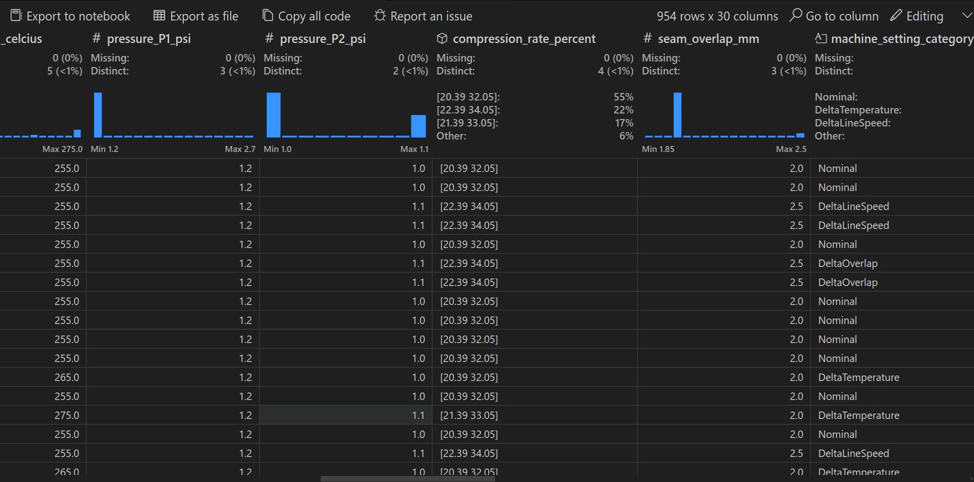
Every row under the `image_data` column contains the bytes of the seam image and there are tens of other columns containing metadata that may be necessary for the subsequent model development.
The `seamagine` dataset is currently a [Map-style dataset](https://pytorch.org/docs/stable/data.html#map-style-datasets) and is compliant with the [Torchvision.datasets API](https://pytorch.org/vision/main/datasets.html).
The dataset table can also be easily visualized interactively using the Data Wrangler VS Code extension.
 ### Split into training and test datasets
The parquet datasets are split into training and test datasets using the `train_test_split` function from the `sklearn` library. The default split ratio is 80:20. The training and test datasets are stored in `seamagine_train.parquet` and `seamagine_test.parquet`. The CLI command `qctl dataset split` splits the dataset into `train` and `test` and uploads the splits to both S3 and Hugging Face Hub.
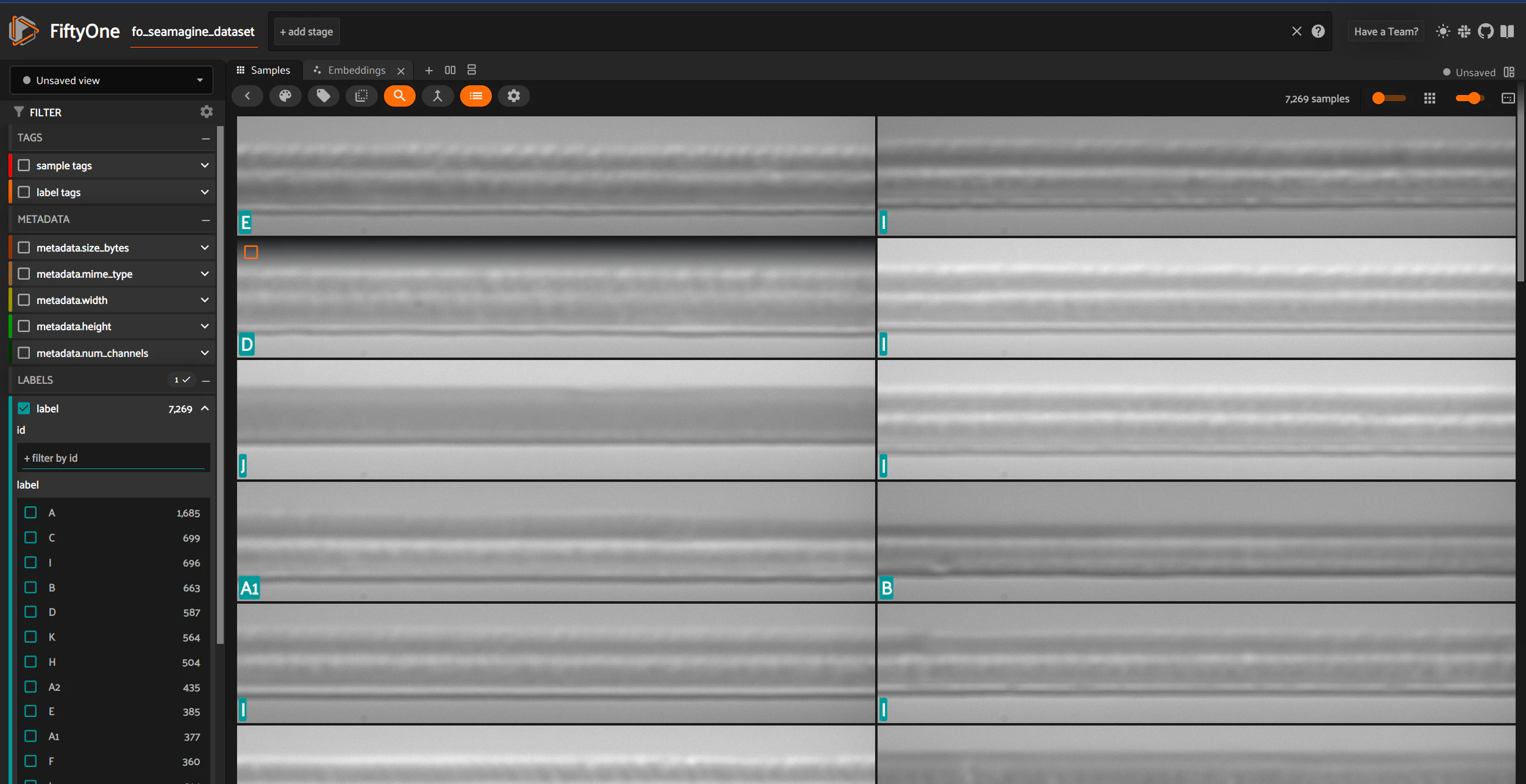
Images can be visualized using the FiftyOne library.
### Split into training and test datasets
The parquet datasets are split into training and test datasets using the `train_test_split` function from the `sklearn` library. The default split ratio is 80:20. The training and test datasets are stored in `seamagine_train.parquet` and `seamagine_test.parquet`. The CLI command `qctl dataset split` splits the dataset into `train` and `test` and uploads the splits to both S3 and Hugging Face Hub.
Images can be visualized using the FiftyOne library.
 ## Dataset Transformations and Statistics
To use the dataset for modeling purposes we need to convert the images to a size that is manageable by any backbone network model based on Convolutional Neural Networks (CNNs). In addition we need to ensure that the network is able to learn the important features from different so called `views` of the images and as a result we apply transformations to the raw images.
### Cropping
We deterministically crop all images from the top and bottom (image height). We then [randomly crop](https://pytorch.org/vision/main/generated/torchvision.transforms.RandomResizedCrop.html) the resultant images with a cropped size of $224 \times 224$ pixels - a common size used in many CNN pretrained models. The randomness in this last cropping ensures that the model "sees" the information across all 1280 pixels of the original images during the duration of the training process that typically lasts for 100s of epochs.
### Flipping
We then perform [RandomHorizontalFlip](https://pytorch.org/vision/stable/generated/torchvision.transforms.RandomHorizontalFlip.html) with the default probability of 0.5.
### Color Jitter
Finally we apply [ColorJitter](https://pytorch.org/vision/stable/transforms.html#torchvision.transforms.ColorJitter) with the following parameters:
* **Brightness**: Adjusted randomly within ±40% of the original brightness.
* **Contrast**: Adjusted randomly within ±40% of the original contrast.
Note that color jitter with just the two parameter adjustments above still maintains the grayscale nature of the images.
### Tensor Conversion
We finally use `torchvision.transforms.ToTensor()` to convert the NumPy array representing an image to a PyTorch tensor. The resulting tensor will have values between 0 and 1.
### Standardization
To ensure that during training we avoid diminishing / exploding gradients that are detrimental to the learning procedure it is common practice to measure the mean and standard deviation per channel (in this case we have only a single color channel) using as input the images *after* the transformations above and populate with the corresponding parameters of the standardization / normalization transformation.
## Anomaly Detection Annotations
From stress test analytics across machine setting categories, the machine setting `C` performed the worst and therefore we decided to use this setting as the `FAIL` or anomalous class for the Anomaly Detection task. We also decided to use only the remaining machine settings within the δT category as the `PASS` class - this includes the `A`, `A1`, `A2`, `B`.
We continue to flag the remaining machine setting categories as `UNDETERMINED`. As we gather additional stress test data, we may vary the mapping of machine setting to either of the two `FAIL` / `PASS` classes. Our implementation allows for flexible mapping of machine settings to classes.
***
[Edit this page on GitHub](https://github.com/aegean-ai/eaia/edit/main/src/products/applications/anomaly-detection/manufacturing/data-pipeline/seamagine.mdx) or [file an issue](https://github.com/aegean-ai/eaia/issues/new/choose).
## Dataset Transformations and Statistics
To use the dataset for modeling purposes we need to convert the images to a size that is manageable by any backbone network model based on Convolutional Neural Networks (CNNs). In addition we need to ensure that the network is able to learn the important features from different so called `views` of the images and as a result we apply transformations to the raw images.
### Cropping
We deterministically crop all images from the top and bottom (image height). We then [randomly crop](https://pytorch.org/vision/main/generated/torchvision.transforms.RandomResizedCrop.html) the resultant images with a cropped size of $224 \times 224$ pixels - a common size used in many CNN pretrained models. The randomness in this last cropping ensures that the model "sees" the information across all 1280 pixels of the original images during the duration of the training process that typically lasts for 100s of epochs.
### Flipping
We then perform [RandomHorizontalFlip](https://pytorch.org/vision/stable/generated/torchvision.transforms.RandomHorizontalFlip.html) with the default probability of 0.5.
### Color Jitter
Finally we apply [ColorJitter](https://pytorch.org/vision/stable/transforms.html#torchvision.transforms.ColorJitter) with the following parameters:
* **Brightness**: Adjusted randomly within ±40% of the original brightness.
* **Contrast**: Adjusted randomly within ±40% of the original contrast.
Note that color jitter with just the two parameter adjustments above still maintains the grayscale nature of the images.
### Tensor Conversion
We finally use `torchvision.transforms.ToTensor()` to convert the NumPy array representing an image to a PyTorch tensor. The resulting tensor will have values between 0 and 1.
### Standardization
To ensure that during training we avoid diminishing / exploding gradients that are detrimental to the learning procedure it is common practice to measure the mean and standard deviation per channel (in this case we have only a single color channel) using as input the images *after* the transformations above and populate with the corresponding parameters of the standardization / normalization transformation.
## Anomaly Detection Annotations
From stress test analytics across machine setting categories, the machine setting `C` performed the worst and therefore we decided to use this setting as the `FAIL` or anomalous class for the Anomaly Detection task. We also decided to use only the remaining machine settings within the δT category as the `PASS` class - this includes the `A`, `A1`, `A2`, `B`.
We continue to flag the remaining machine setting categories as `UNDETERMINED`. As we gather additional stress test data, we may vary the mapping of machine setting to either of the two `FAIL` / `PASS` classes. Our implementation allows for flexible mapping of machine settings to classes.
***
[Edit this page on GitHub](https://github.com/aegean-ai/eaia/edit/main/src/products/applications/anomaly-detection/manufacturing/data-pipeline/seamagine.mdx) or [file an issue](https://github.com/aegean-ai/eaia/issues/new/choose).