Open In Colab

Behavioral Cloning with CarRacing-v3

Behavioral cloning (BC) is the simplest form of imitation learning: collect expert demonstrations, then train a policy via supervised learning to map observations to actions. It is the starting point for understanding why imitation learning works — and why it fails. In this notebook you will:
  1. Train an expert policy using PPO
  2. Collect expert driving demonstrations
  3. Train a BC policy via supervised learning on the expert’s data
  4. Observe distribution shift — the core failure mode of BC
  5. Fix it with DAgger (Dataset Aggregation)
Environment: CarRacing-v3 — a continuous-control driving task where the agent observes a 96×96 RGB top-down view of a procedurally generated race track and outputs steering, throttle, and brake.

Setup

!pip install -q "gymnasium[box2d]" stable-baselines3 swig rich tqdm
import gymnasium as gym
import numpy as np
import matplotlib.pyplot as plt
import torch
import torch.nn as nn
import torch.optim as optim
from torch.utils.data import DataLoader, TensorDataset
from stable_baselines3 import PPO
from stable_baselines3.common.vec_env import DummyVecEnv, SubprocVecEnv
from stable_baselines3.common.evaluation import evaluate_policy

SEED = 42
np.random.seed(SEED)
torch.manual_seed(SEED)
device = torch.device("cuda" if torch.cuda.is_available() else "cpu")
print(f"Device: {device}")
Device: cuda

Step 1: Create the environment

def make_env():
    return gym.make("CarRacing-v3", continuous=True, render_mode="rgb_array")

# Parallel envs for fast PPO rollout collection
N_TRAIN_ENVS = 8
train_venv = SubprocVecEnv([make_env for _ in range(N_TRAIN_ENVS)])

# Single env for evaluation and demo collection (simpler to read)
venv = DummyVecEnv([make_env])

print(f"Train envs:    {N_TRAIN_ENVS} parallel (SubprocVecEnv)")
print(f"Eval env:      1 (DummyVecEnv)")
print(f"Observation:   {venv.observation_space}")
print(f"Action:        {venv.action_space}")
Train envs:    8 parallel (SubprocVecEnv)
Eval env:      1 (DummyVecEnv)
Observation:   Box(0, 255, (96, 96, 3), uint8)
Action:        Box([-1.  0.  0.], 1.0, (3,), float32)
/home/pantelis.monogioudis/repos/eng-ai-agents/.venv/lib/python3.12/site-packages/pygame/pkgdata.py:25: UserWarning: pkg_resources is deprecated as an API. See https://setuptools.pypa.io/en/latest/pkg_resources.html. The pkg_resources package is slated for removal as early as 2025-11-30. Refrain from using this package or pin to Setuptools<81.
  from pkg_resources import resource_stream, resource_exists

Step 2: Train an expert policy

We train an expert using PPO. In a real setting you might use a pre-trained checkpoint or human teleoperation. Here PPO acts as our “expert driver.” Note: Training for 200k timesteps takes ~5-10 minutes on CPU.
from stable_baselines3.common.callbacks import BaseCallback


class TrainingMetricsCallback(BaseCallback):
    """Capture key PPO training metrics after each rollout for later plotting."""

    def __init__(self):
        super().__init__()
        self.timesteps = []
        self.std = []
        self.value_loss = []
        self.explained_variance = []
        self.entropy_loss = []
        self.policy_gradient_loss = []
        self.approx_kl = []
        self.clip_fraction = []

    def _on_step(self) -> bool:
        return True

    def _on_rollout_end(self) -> None:
        # Pull metrics from the SB3 logger after each rollout-and-update
        log = self.logger.name_to_value
        self.timesteps.append(self.num_timesteps)
        # std is stored under "train/std" once a Gaussian distribution is used
        self.std.append(log.get("train/std", float("nan")))
        self.value_loss.append(log.get("train/value_loss", float("nan")))
        self.explained_variance.append(log.get("train/explained_variance", float("nan")))
        self.entropy_loss.append(log.get("train/entropy_loss", float("nan")))
        self.policy_gradient_loss.append(log.get("train/policy_gradient_loss", float("nan")))
        self.approx_kl.append(log.get("train/approx_kl", float("nan")))
        self.clip_fraction.append(log.get("train/clip_fraction", float("nan")))


expert = PPO(
    "CnnPolicy",
    train_venv,
    verbose=0,
    seed=SEED,
    n_steps=512,
    batch_size=256,
    n_epochs=10,
    learning_rate=3e-4,
)

metrics_cb = TrainingMetricsCallback()

# 200k total timesteps across 8 parallel envs = 25k env steps wall-clock
expert.learn(total_timesteps=200_000, progress_bar=True, callback=metrics_cb)
print("Expert training complete")
/home/pantelis.monogioudis/repos/eng-ai-agents/.venv/lib/python3.12/site-packages/rich/live.py:260: UserWarning: 
install "ipywidgets" for Jupyter support
  warnings.warn('install "ipywidgets" for Jupyter support')
Expert training complete

Reading PPO training output

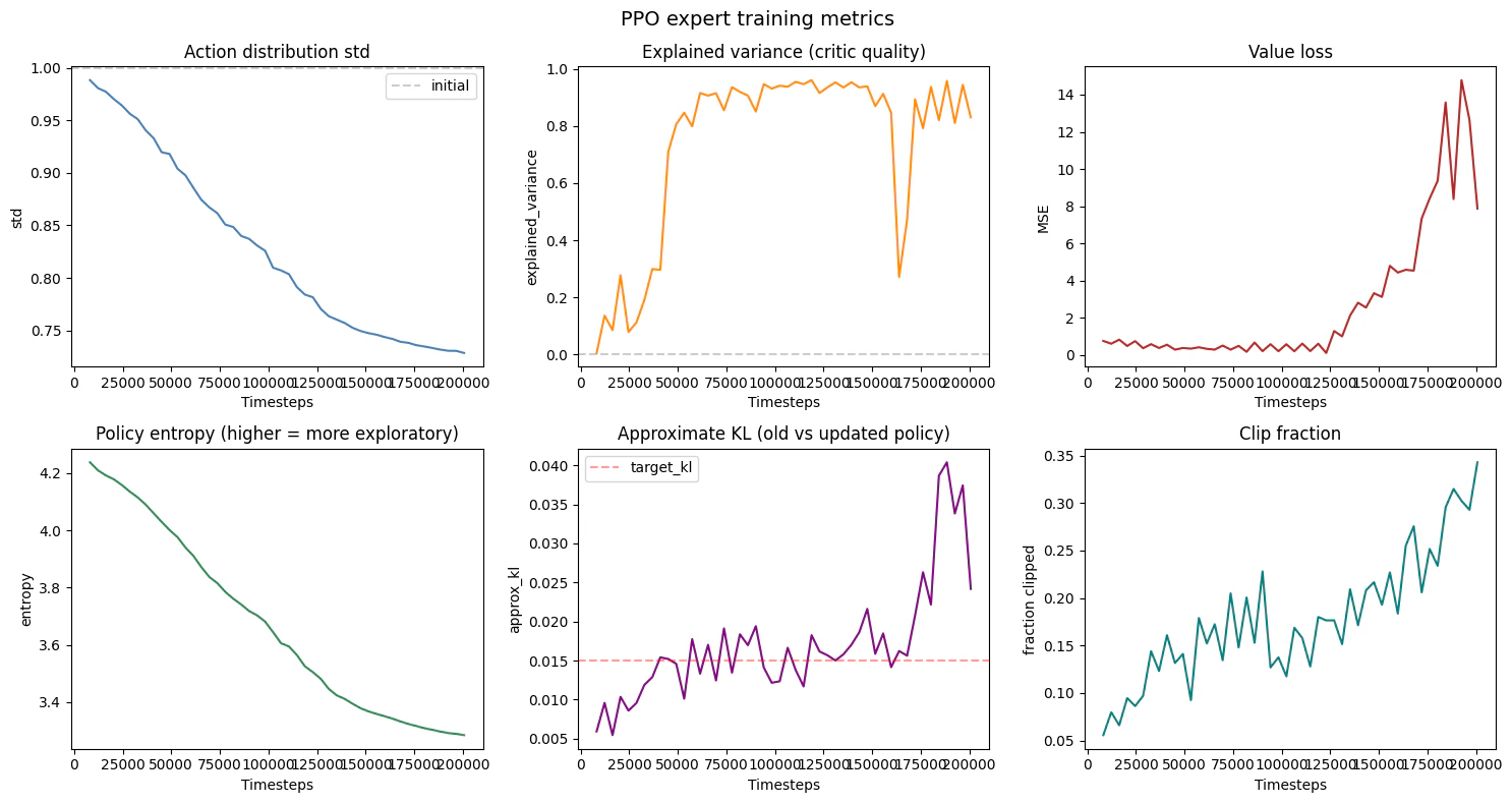
PPO logs a block of metrics after each rollout-and-update iteration. With verbose=1 you would see something like this:
-----------------------------------------
| time/                   |             |
|    fps                  | 124         |
|    iterations           | 2           |
|    time_elapsed         | 16          |
|    total_timesteps      | 2048        |
| train/                  |             |
|    approx_kl            | 0.007264021 |
|    clip_fraction        | 0.0696      |
|    clip_range           | 0.2         |
|    entropy_loss         | -4.25       |
|    explained_variance   | 0.0162      |
|    learning_rate        | 0.0003      |
|    loss                 | 0.393       |
|    n_updates            | 10          |
|    policy_gradient_loss | -0.00708    |
|    std                  | 0.994       |
|    value_loss           | 0.811       |
-----------------------------------------
PPO uses a diagonal Gaussian action distribution for continuous control: the CNN outputs the mean of each action dimension, and the standard deviation (std) is a separate learned parameter (state-independent log_std). Actions are sampled from Normal(mean, std) at training time and set to mean at evaluation time when deterministic=True. There is no diffusion head — modern diffusion-based action heads (Chi et al. 2023) are an alternative used in some manipulation BC systems, but they are not required for continuous control and SB3 PPO does not use them. Each metric and the trend you should expect during a healthy run:
MetricMeaningHealthy trend
fpsEnvironment steps per second across all parallel workersRoughly constant; depends on hardware
total_timestepsCumulative env steps consumedMonotonic
approx_klKL between old and updated policy after the gradient stepsStays below ~0.02; spikes mean the policy moved too far
clip_fractionFraction of samples whose probability ratio was clipped by PPO’s surrogate0.0 - 0.3 is normal; >0.5 means too-aggressive updates
entropy_lossNegative entropy of the action distribution (PPO maximises entropy)Becomes less negative as the policy commits
explained_varianceHow well the value head predicts returnsShould rise from 0 toward 0.5 - 0.9
policy_gradient_lossClipped surrogate loss being minimisedSmall magnitude, can be slightly negative
stdStandard deviation of the Gaussian action distributionDrops from ~1.0 toward ~0.1 - 0.3 as the policy commits
value_lossMSE between value head prediction and actual returnDecreases as explained_variance rises
The next cell plots these metrics over the course of training using the data captured by the callback above.
fig, axes = plt.subplots(2, 3, figsize=(15, 8))
ts = metrics_cb.timesteps

axes[0, 0].plot(ts, metrics_cb.std, color="steelblue")
axes[0, 0].set_title("Action distribution std")
axes[0, 0].set_xlabel("Timesteps")
axes[0, 0].set_ylabel("std")
axes[0, 0].axhline(y=1.0, color="gray", linestyle="--", alpha=0.4, label="initial")
axes[0, 0].legend()

axes[0, 1].plot(ts, metrics_cb.explained_variance, color="darkorange")
axes[0, 1].set_title("Explained variance (critic quality)")
axes[0, 1].set_xlabel("Timesteps")
axes[0, 1].set_ylabel("explained_variance")
axes[0, 1].axhline(y=0.0, color="gray", linestyle="--", alpha=0.4)

axes[0, 2].plot(ts, metrics_cb.value_loss, color="firebrick")
axes[0, 2].set_title("Value loss")
axes[0, 2].set_xlabel("Timesteps")
axes[0, 2].set_ylabel("MSE")

axes[1, 0].plot(ts, [-e for e in metrics_cb.entropy_loss], color="seagreen")
axes[1, 0].set_title("Policy entropy (higher = more exploratory)")
axes[1, 0].set_xlabel("Timesteps")
axes[1, 0].set_ylabel("entropy")

axes[1, 1].plot(ts, metrics_cb.approx_kl, color="purple")
axes[1, 1].set_title("Approximate KL (old vs updated policy)")
axes[1, 1].set_xlabel("Timesteps")
axes[1, 1].set_ylabel("approx_kl")
axes[1, 1].axhline(y=0.015, color="red", linestyle="--", alpha=0.4, label="target_kl")
axes[1, 1].legend()

axes[1, 2].plot(ts, metrics_cb.clip_fraction, color="teal")
axes[1, 2].set_title("Clip fraction")
axes[1, 2].set_xlabel("Timesteps")
axes[1, 2].set_ylabel("fraction clipped")

fig.suptitle("PPO expert training metrics", fontsize=14)
plt.tight_layout()
plt.show()
Output from cell 5
expert_reward, expert_std = evaluate_policy(expert, venv, n_eval_episodes=10)
print(f"Expert mean reward: {expert_reward:.1f} +/- {expert_std:.1f}")
/home/pantelis.monogioudis/repos/eng-ai-agents/.venv/lib/python3.12/site-packages/stable_baselines3/common/evaluation.py:71: UserWarning: Evaluation environment is not wrapped with a ``Monitor`` wrapper. This may result in reporting modified episode lengths and rewards, if other wrappers happen to modify these. Consider wrapping environment first with ``Monitor`` wrapper.
  warnings.warn(
Expert mean reward: 347.3 +/- 223.3

Step 3: Collect expert demonstrations

Roll out the expert to collect (observation, action) pairs — this is our training data for behavioral cloning.
def collect_demonstrations(policy, venv, n_episodes=50):
    """Collect (obs, action) pairs from a policy."""
    all_obs, all_actions = [], []
    for ep in range(n_episodes):
        obs = venv.reset()
        done = False
        while not done:
            action, _ = policy.predict(obs, deterministic=True)
            all_obs.append(obs[0].copy())
            all_actions.append(action[0].copy())
            obs, reward, done, info = venv.step(action)
    return np.array(all_obs), np.array(all_actions)

expert_obs, expert_actions = collect_demonstrations(expert, venv, n_episodes=50)
print(f"Collected {len(expert_obs)} transitions from 50 episodes")
print(f"Observation shape: {expert_obs.shape}")
print(f"Action shape: {expert_actions.shape}")

# Show sample observations
fig, axes = plt.subplots(1, 4, figsize=(12, 3))
for i, ax in enumerate(axes):
    idx = i * (len(expert_obs) // 4)
    ax.imshow(expert_obs[idx])
    ax.set_title(f"Frame {idx}")
    ax.axis("off")
fig.suptitle("Sample expert observations")
plt.tight_layout()
plt.show()
Collected 38431 transitions from 50 episodes
Observation shape: (38431, 96, 96, 3)
Action shape: (38431, 3)
Output from cell 7

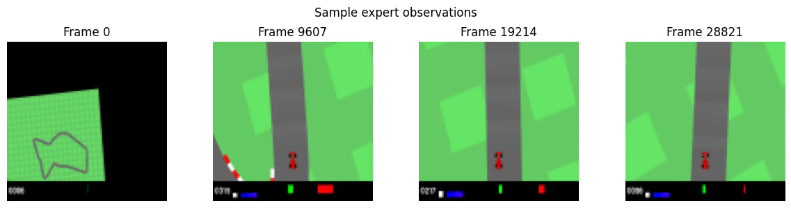
Step 4: Train a behavioral cloning policy

BC is supervised learning: a CNN maps observations to actions, trained with MSE loss against the expert’s recorded actions.
class BCPolicy(nn.Module):
    """CNN policy that maps 96x96 RGB observations to 3 continuous actions."""

    def __init__(self):
        super().__init__()
        # Input: (batch, 96, 96, 3) -> permute to (batch, 3, 96, 96)
        self.features = nn.Sequential(
            nn.Conv2d(3, 32, 8, stride=4),
            nn.ReLU(),
            nn.Conv2d(32, 64, 4, stride=2),
            nn.ReLU(),
            nn.Conv2d(64, 64, 3, stride=1),
            nn.ReLU(),
            nn.Flatten(),
        )
        # Calculate flattened size
        with torch.no_grad():
            dummy = torch.zeros(1, 3, 96, 96)
            n_flat = self.features(dummy).shape[1]

        self.head = nn.Sequential(
            nn.Linear(n_flat, 256),
            nn.ReLU(),
            nn.Linear(256, 3),  # steering, throttle, brake
            nn.Tanh(),  # actions in [-1, 1]
        )

    def forward(self, x):
        # x: (batch, H, W, C) uint8 -> (batch, C, H, W) float32
        if x.dim() == 3:
            x = x.unsqueeze(0)
        x = x.permute(0, 3, 1, 2).float() / 255.0
        return self.head(self.features(x))

bc_policy = BCPolicy().to(device)
print(f"BC policy parameters: {sum(p.numel() for p in bc_policy.parameters()):,}")
BC policy parameters: 1,125,539
# Prepare data
obs_tensor = torch.tensor(expert_obs, dtype=torch.uint8)
act_tensor = torch.tensor(expert_actions, dtype=torch.float32)

dataset = TensorDataset(obs_tensor, act_tensor)
dataloader = DataLoader(dataset, batch_size=64, shuffle=True)

# Train
optimizer = optim.Adam(bc_policy.parameters(), lr=3e-4)
loss_fn = nn.MSELoss()

losses = []
for epoch in range(20):
    epoch_loss = 0
    for obs_batch, act_batch in dataloader:
        obs_batch = obs_batch.to(device)
        act_batch = act_batch.to(device)

        pred_actions = bc_policy(obs_batch)
        loss = loss_fn(pred_actions, act_batch)

        optimizer.zero_grad()
        loss.backward()
        optimizer.step()
        epoch_loss += loss.item()

    avg_loss = epoch_loss / len(dataloader)
    losses.append(avg_loss)
    if (epoch + 1) % 5 == 0:
        print(f"Epoch {epoch+1:2d}/20  loss={avg_loss:.4f}")

plt.figure(figsize=(8, 3))
plt.plot(losses)
plt.xlabel("Epoch")
plt.ylabel("MSE Loss")
plt.title("BC Training Loss")
plt.tight_layout()
plt.show()
Epoch  5/20  loss=0.0026
Epoch 10/20  loss=0.0015
Epoch 15/20  loss=0.0011
Epoch 20/20  loss=0.0008
Output from cell 9

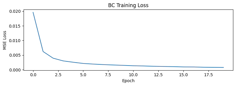
Step 5: Evaluate and observe distribution shift

Deploy the BC policy and compare against the expert. What you will observe: the BC policy performs noticeably worse than the expert. On straight sections it may track the road, but on sharp turns it drifts off. Once off-track, it enters states the expert never demonstrated — predictions become unreliable, and the car spirals further off course. This is compounding error from distribution shift: at training time, the policy only saw states along the expert’s trajectory. At test time, any small deviation puts the agent in unfamiliar territory.
def evaluate_bc(policy, venv, n_episodes=20):
    """Evaluate a PyTorch BC policy in the vectorized env."""
    rewards = []
    for _ in range(n_episodes):
        obs = venv.reset()
        total_reward = 0
        done = False
        while not done:
            with torch.no_grad():
                obs_t = torch.tensor(obs[0], dtype=torch.uint8).to(device)
                action = policy(obs_t).cpu().numpy().flatten()
            obs, reward, done, info = venv.step([action])
            total_reward += reward[0]
        rewards.append(total_reward)
    return rewards

def evaluate_sb3(policy, venv, n_episodes=20):
    """Evaluate an SB3 policy."""
    rewards = []
    for _ in range(n_episodes):
        obs = venv.reset()
        total_reward = 0
        done = False
        while not done:
            action, _ = policy.predict(obs, deterministic=True)
            obs, reward, done, info = venv.step(action)
            total_reward += reward[0]
        rewards.append(total_reward)
    return rewards

expert_rewards = evaluate_sb3(expert, venv, n_episodes=20)
bc_rewards = evaluate_bc(bc_policy, venv, n_episodes=20)

print(f"Expert: {np.mean(expert_rewards):.1f} +/- {np.std(expert_rewards):.1f}")
print(f"BC:     {np.mean(bc_rewards):.1f} +/- {np.std(bc_rewards):.1f}")

fig, ax = plt.subplots(figsize=(8, 4))
ax.boxplot([expert_rewards, bc_rewards], labels=["Expert (PPO)", "Behavioral Cloning"])
ax.set_ylabel("Episode Reward")
ax.set_title("Expert vs BC: Distribution Shift Degrades Performance")
ax.axhline(y=0, color="gray", linestyle="--", alpha=0.5)
plt.tight_layout()
plt.show()
Expert: 416.4 +/- 271.9
BC:     441.7 +/- 239.8
/tmp/ipykernel_3614068/1622135918.py:38: MatplotlibDeprecationWarning: The 'labels' parameter of boxplot() has been renamed 'tick_labels' since Matplotlib 3.9; support for the old name will be dropped in 3.11.
  ax.boxplot([expert_rewards, bc_rewards], labels=["Expert (PPO)", "Behavioral Cloning"])
Output from cell 10

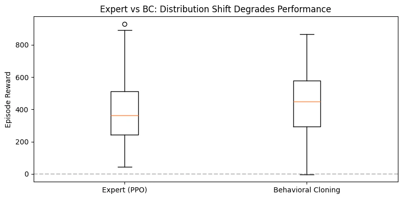
Step 6: Fix it with DAgger

DAgger (Dataset Aggregation) addresses distribution shift by iteratively collecting new data from the learner’s trajectory, labeled by the expert. The algorithm:
  1. Train an initial BC policy on expert demonstrations
  2. Roll out the learner’s policy in the environment
  3. Ask the expert to label the states the learner visited (what would you have done here?)
  4. Add this new data to the training set
  5. Retrain and repeat
def dagger_round(bc_policy, expert, venv, n_episodes=10):
    """Run one round of DAgger: roll out the learner, label with expert."""
    new_obs, new_actions = [], []
    for _ in range(n_episodes):
        obs = venv.reset()
        done = False
        while not done:
            # Learner drives
            with torch.no_grad():
                obs_t = torch.tensor(obs[0], dtype=torch.uint8).to(device)
                learner_action = bc_policy(obs_t).cpu().numpy().flatten()

            # Expert labels what IT would have done in this state
            expert_action, _ = expert.predict(obs, deterministic=True)

            new_obs.append(obs[0].copy())
            new_actions.append(expert_action[0].copy())

            # Learner's action determines next state
            obs, reward, done, info = venv.step([learner_action])

    return np.array(new_obs), np.array(new_actions)


def train_bc_on_data(bc_policy, all_obs, all_actions, n_epochs=5, lr=1e-4):
    """Retrain BC policy on accumulated data."""
    dataset = TensorDataset(
        torch.tensor(all_obs, dtype=torch.uint8),
        torch.tensor(all_actions, dtype=torch.float32),
    )
    loader = DataLoader(dataset, batch_size=64, shuffle=True)
    optimizer = optim.Adam(bc_policy.parameters(), lr=lr)
    loss_fn = nn.MSELoss()

    for epoch in range(n_epochs):
        for obs_batch, act_batch in loader:
            pred = bc_policy(obs_batch.to(device))
            loss = loss_fn(pred, act_batch.to(device))
            optimizer.zero_grad()
            loss.backward()
            optimizer.step()


# Start DAgger with the original expert data
all_obs = expert_obs.copy()
all_actions = expert_actions.copy()

# Reset BC policy for fair comparison
dagger_policy = BCPolicy().to(device)

# Initial BC training
train_bc_on_data(dagger_policy, all_obs, all_actions, n_epochs=20, lr=3e-4)

dagger_progress = []
N_ROUNDS = 5

for r in range(N_ROUNDS):
    # Collect new data from learner's trajectory, labeled by expert
    new_obs, new_actions = dagger_round(dagger_policy, expert, venv, n_episodes=10)

    # Aggregate
    all_obs = np.concatenate([all_obs, new_obs])
    all_actions = np.concatenate([all_actions, new_actions])

    # Retrain on full dataset
    train_bc_on_data(dagger_policy, all_obs, all_actions, n_epochs=5, lr=1e-4)

    # Evaluate
    rewards = evaluate_bc(dagger_policy, venv, n_episodes=10)
    mean_r = np.mean(rewards)
    dagger_progress.append(mean_r)
    print(f"DAgger round {r+1}/{N_ROUNDS}  data={len(all_obs):,}  reward={mean_r:.1f}")

print(f"\nFinal dataset size: {len(all_obs):,} transitions")
DAgger round 1/5  data=45,869  reward=418.6
DAgger round 2/5  data=54,312  reward=338.0
DAgger round 3/5  data=62,887  reward=294.5
DAgger round 4/5  data=71,650  reward=302.5
DAgger round 5/5  data=80,023  reward=288.8

Final dataset size: 80,023 transitions

Compare all three policies
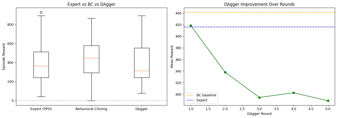
dagger_rewards = evaluate_bc(dagger_policy, venv, n_episodes=20)

print(f"Expert: {np.mean(expert_rewards):.1f} +/- {np.std(expert_rewards):.1f}")
print(f"BC:     {np.mean(bc_rewards):.1f} +/- {np.std(bc_rewards):.1f}")
print(f"DAgger: {np.mean(dagger_rewards):.1f} +/- {np.std(dagger_rewards):.1f}")

fig, (ax1, ax2) = plt.subplots(1, 2, figsize=(14, 5))

# Box plot comparison
ax1.boxplot(
    [expert_rewards, bc_rewards, dagger_rewards],
    labels=["Expert (PPO)", "Behavioral Cloning", "DAgger"],
)
ax1.set_ylabel("Episode Reward")
ax1.set_title("Expert vs BC vs DAgger")
ax1.axhline(y=0, color="gray", linestyle="--", alpha=0.5)

# DAgger learning curve
ax2.plot(range(1, N_ROUNDS + 1), dagger_progress, "o-", color="green")
ax2.axhline(y=np.mean(bc_rewards), color="orange", linestyle="--", label="BC baseline")
ax2.axhline(y=np.mean(expert_rewards), color="blue", linestyle="--", label="Expert")
ax2.set_xlabel("DAgger Round")
ax2.set_ylabel("Mean Reward")
ax2.set_title("DAgger Improvement Over Rounds")
ax2.legend()

plt.tight_layout()
plt.show()
Expert: 416.4 +/- 271.9
BC:     441.7 +/- 239.8
DAgger: 385.0 +/- 235.1
/tmp/ipykernel_3614068/1566362.py:10: MatplotlibDeprecationWarning: The 'labels' parameter of boxplot() has been renamed 'tick_labels' since Matplotlib 3.9; support for the old name will be dropped in 3.11.
  ax1.boxplot(
Output from cell 12

Summary

PolicyTraining methodDistribution shift?
Expert (PPO)RL with environment rewardN/A — defines the target distribution
Behavioral CloningSupervised regression on expert dataYes — compounds errors on unseen states
DAggerIterative BC with learner-visited states labeled by expertMitigated — training distribution converges to test distribution
The distribution shift problem you observed here — and DAgger’s fix of relabeling learner-visited states — reappears throughout robot learning. Later in the course, you will revisit these ideas in the context of world models and VLA architectures, where the same fundamental challenge is addressed at larger scale.

Further reading