Let me introduce you MIT prof G Strang - probably the best educator in America. He has published this playlist of youtube videos on Linear Algebra. Also, watch these videos for a more elementary treatment of the topic.
Linear Algebra recitation for my classes. Recitation was delivered by my TA Shweta Selvaraj Achary. The corresponding chapter of Ian Goodfellow’s Deep Learning book is what you partially need to know as data scientists at a graduate level but arguably if you are just starting you ought to know 2.1-2.5.

Key Points

We can now summarize the points to pay attention to, for ML applications. In the following we assume a data matrix AA with mm rows and nn columns. We also assume that the matrix is such that it has rr independent rows or columns, called the matrix rank.

Projections

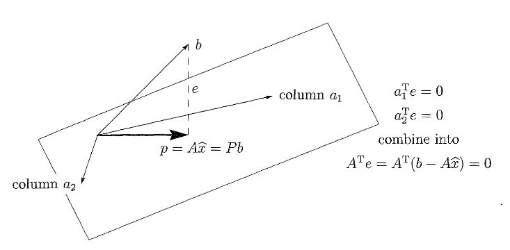
Its important to understand this basic operator and its geometric interpretation as it is met in problems like Ordinary Least Squares but also all over ML and other fields such as compressed sensing. In the following we assume that the reader is familiar with the concept of vector spaces and subspaces. Let SS be a vector subspace of RnR^n. For example in R3R^3, SS are the lines and planes going through the origin. The projection operator onto SS implements a linear transformation: ΠS:R3S\Pi_S: R^3 →S. We will stick to R3R^3 to maintain the ability to plot the operations involved. We also define the orthogonal subspace, S{wR3wTs=0,sS}S^\perp \equiv \{ \mathbf{w} \in \mathbb{R}^3 \mid \mathbf{w}^T \mathbf{s} = 0, \forall \mathbf{s} \in S \} The transformation ΠS\Pi_S projects onto space SS in the sense that when you apply this operator, every vector u\mathbf u in any other space results in the subspace SS. In our example above, ΠS(u)S,uR3\Pi_S(\mathbf u) \in S, \forall \mathbf u \in R^3 This means that any components of the vector u\mathbf u that belonged to SS^\perp are gone when applying the projection operator. Effectively, the original space is decomposed into R3=SSR^3 = S \oplus S^\perp Now we can treat projections onto specific subspaces such as lines and planes passing through the origin. For a line defined by a direction vector u\mathbf u l={(x,y,z)R3(x,y,z)=0+tu}l = \{ (x,y,z) \in \mathbb{R}^3 \mid (x,y,z) = \mathbf{0} + t \mathbf{u} \} we can define the projection onto the line line-projection Projection of u\mathbf u onto the line ll The space SlS^\perp ≡ l^\perp is a plane since it consists of all the vectors that are perpendicular to the line. What is shown in the figure as a dashed line is simply the projection of u\mathbf u on the ll^\perp subspace, l={(x,y,z)R3[xyz]Tv=0}l^\perp = \{ (x,y,z) \in \mathbb{R}^3 \mid \begin{bmatrix} x \\ y \\ z \end{bmatrix}^T \mathbf{v} = 0 \} The orthogonal space of a line with direction vector v\mathbf v is a plane with a normal vector v\mathbf v. So when we project the v\mathbf v on the line we get two components one is lying on the line and is the Πlu\Pi_l \mathbf u and the other is the vector w\mathbf w = Πlu=uv=uΠvu\Pi_{l^\perp} \mathbf u = \mathbf u - \mathbf v = \mathbf u - \Pi_{\mathbf v} \mathbf u . The vector w\mathbf w is what remains when we remove the projected on v\mathbf v part from the u\mathbf u.

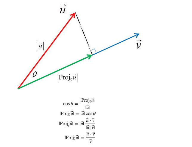
The Four Fundamental Subspaces
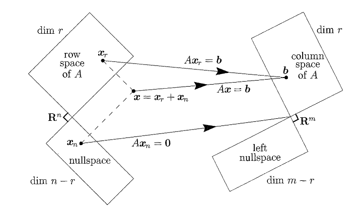
Four fundamental spaces The fundamental theorem of Linear Algebra specifies the effect of the multiplication operation of the matrix and a vector (AxA\mathbf{x}). The matrix gives raise to 4 subspaces:
  1. The column space of AA, denoted by R(A)\mathcal{R}(A), with dimension rr.
  2. The nullspace of AA, denoted by N(A)\mathcal{N}(A), with dimension nrn-r.
  3. The row space of AA which is the column space of ATA^T, with dimension rr
  4. The left nullspace of AA, which is the nullspace of ATA^T, denoted by N(AT)\mathcal{N}(A^T), with dimension mrm-r.
The real action that the matrix performs is to transform its row space to its column space. The type of matrices that are common in ML are those that the number of rows mm representing observations is much larger than the number of columns nn that represent features. We will call these matrices “tall” for obvious reasons. Let us consider one trivial but instructive example of the smallest possible “tall” matrix: [a11a12a21a22a31a32]=[105424]\begin{bmatrix} a_{11} & a_{12} \\ a_{21} & a_{22} \\ a_{31} & a_{32} \end{bmatrix} = \begin{bmatrix} 1 & 0 \\ 5 & 4 \\ 2 & 4 \end{bmatrix} In ML we are usually concerned with the problem of learning the weights x1,x2x_1, x_2 that will combine the features and result into the given target variables b\mathbf{b}. The notation here is different and we have adopted the notation of many linear algebra textbooks. \begin\{bmatrix\} b_1 \\ b_2 \\ b_3 \end\{bmatrix\}$$ To make more explicit the combination of features we can write, $$ x_1 \begin{bmatrix} 1 \\ 5 \\ 2 \end{bmatrix} + x_2 \begin{bmatrix} 0 \\ 4 \\ 4 \end{bmatrix} = \begin{bmatrix} b_1 \\ b_2 \\ b_3 \end{bmatrix}$$ Since $m=3 > n=2$, we have more equations than unknowns we in general we have no solutions - a system with $m > n$ will be solvable only for certain right hand sides $\mathbf{b}$. Those are all the vectors $\mathbf{b}$ that lie in the column space of $A$. ![column-space](/aiml-common/lectures/ml-math/linear-algebra/images/column-space.png) In this example, as shown in the picture $\mathbf{b}$ must lie in the plane spanned by the two columns of $A$. The plane is a subspace of $\mathbb{R}^m=\mathbb{R}^3$ in this case. Now instead of looking at what properties $\mathbf{b}$ must have for the system to have a solution, lets look at the *dual* problem i.e. what weights $\mathbf{x}$ can attain those $\mathbf{b}$. The right-hand side $\mathbf{b}=0$ always allows the solution $\mathbf{x}=0$ The solutions to $A \mathbf{x} = \mathbf{0}$ form a vector space - **the nullspace** $\mathcal{N}(A)$. The nullspace is also called the *kernel* of matrix $A$ and the its dimension $n-r$ is called the nullity. $\mathcal{N}(A)$ is a subspace of $\mathbb{R}^n=\mathbb{R}^2$ in this case. For our specific example, $$ x_1 \begin{bmatrix} 1 \\ 5 \\ 2 \end{bmatrix} + x_2 \begin{bmatrix} 0 \\ 4 \\ 4 \end{bmatrix} = \begin{bmatrix} 0 \\ 0 \\ 0 \end{bmatrix}$$ the only solution that can satisfy this set of homogenous equations is: $\mathbf{x}=\mathbf{0}$ and this means that the null space contains only the zero vector and this Two vectors are independent when their linear combination cannot be zero, unless both $x_1$ and $x_2$ are zero. The columns of $A$ are therefore linearly independent and they span the column space. They have therefore all the properties needed for them to constitute a set called the *basis* for that space and we have two basis vectors (the rank is $r=2$ in this case). The dimension of the column space is in fact the same as the dimension of the row space ($r$) and the mapping from row space to column space is in fact invertible. Every vector $\mathbf{b}$ comes from one and only one vector $\mathbf{x}$ of the row space ($\mathbf{x}_r$). And this vector can be found by the inverse operation - noting that only the inverse $A^{-1}$ is the operation that moves the vector correctly from the column space to the row space. The inverse exists only if $r=m=n$ - this is important as in most ML problems we are dealing with "tall" matrices with the number of equations much larger than the number of unknowns which makes the system *inconsistent* (or *degenerate*). ![projection-column-space](/aiml-common/lectures/ml-math/linear-algebra/images/projection-column-space.png) *Projection onto the column space* Geometrically you can think about the basis vectors as the axes of the space. However, if the axes are not orthogonal, calculations will tend to be complicated not to mention that we usually attribute to each vector of the basis to have length one (1.0). ### 
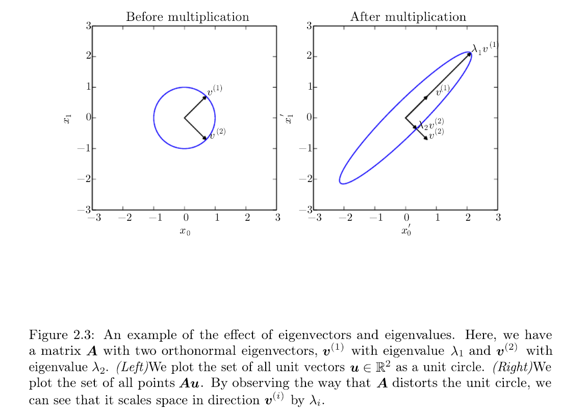
Eigenvalues and Eigenvectors The following video gives an intuitive explanation of eigenvalues and eigenvectors and its included here due to its visualizations that it offers. The video must be viewed in conjunction with [Strang's introduction](http://math.mit.edu/~gs/linearalgebra/linearalgebra5_6-1.pdf) <iframe width="560" height="315" src="https://www.youtube.com/embed/PFDu9oVAE-g" frameborder="0" allow="accelerometer; autoplay; encrypted-media; gyroscope; picture-in-picture" allowfullscreen></iframe> A geometric interpretation of the eigenvectors and eigenvalues is given in the following figure: ![eigenvectors](/aiml-common/lectures/ml-math/linear-algebra/images/eigenvectors.png) --- <Callout icon="pen-to-square" iconType="regular"> [Edit this page on GitHub](https://github.com/langchain-ai/docs/edit/main/src/aiml-common/lectures/ml-math/linear-algebra/index.mdx) or [file an issue](https://github.com/langchain-ai/docs/issues/new/choose). </Callout> <Tip icon="terminal" iconType="regular"> [Connect these docs](/use-these-docs) to Claude, VSCode, and more via MCP for real-time answers. </Tip>