
Odometry Motion Model

Odometry is commonly obtained by integrating wheel encoders information; most commercial robots make such integrated pose estimation available in periodic time intervals (e.g., every tenth of a second).
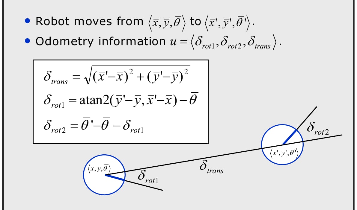
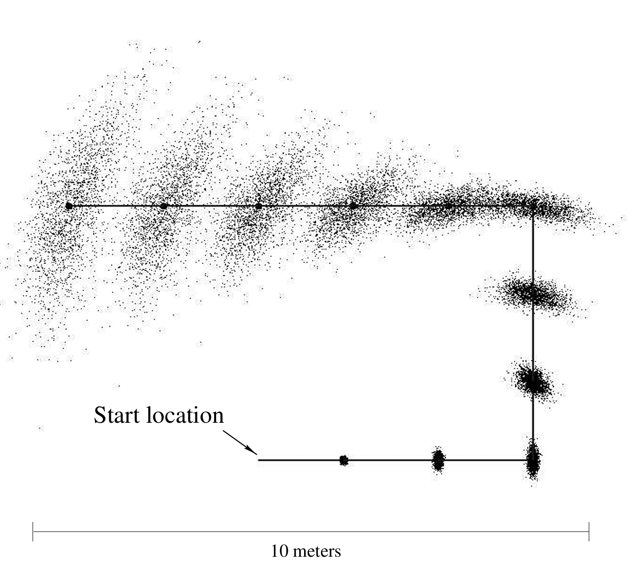
 Odometry model Measured Odometry model Sampled Odometry model Odometry belief over time Wheel displacements derived from encoder readings produce noisy pose update: p(xtxt1,ut)=p(Δrot1^)p(Δtrans^)p(Δrot2^),p(x_t \mid x_{t-1}, u_t) = p(\widehat{\Delta_{\text{rot}_1}}) \, p(\widehat{\Delta_{\text{trans}}}) \, p(\widehat{\Delta_{\text{rot}_2}}), factorized by initial rotation, translation, final rotation. Compute noisy components: Δrot1=atan2(ytyt1,xtxt1)θt1\Delta_{\text{rot}_1} = \operatorname{atan2}(y_t - y_{t-1}, x_t - x_{t-1}) - \theta_{t-1} Δtrans=(xtxt1)2+(ytyt1)2\Delta_{\text{trans}} = \sqrt{(x_t - x_{t-1})^2 + (y_t - y_{t-1})^2} Δrot2=θtθt1Δrot1\Delta_{\text{rot}_2} = \theta_t - \theta_{t-1} - \Delta_{\text{rot}_1} Sample corrupted increments: Δrot1~=Δrot1N(0,α1Δrot12+α2Δtrans2)\widetilde{\Delta_{\text{rot}_1}} = \Delta_{\text{rot}_1} - \mathcal{N}(0, \alpha_1 \Delta_{\text{rot}_1}^2 + \alpha_2 \Delta_{\text{trans}}^2) and similarly for Δtrans~\widetilde{\Delta_{\text{trans}}} and Δrot2~\widetilde{\Delta_{\text{rot}_2}}. Updated pose: xt=xt1+Δtrans~cos(θt1+Δrot1~)x_t = x_{t-1} + \widetilde{\Delta_{\text{trans}}} \cos(\theta_{t-1} + \widetilde{\Delta_{\text{rot}_1}}) yt=yt1+Δtrans~sin(θt1+Δrot1~)y_t = y_{t-1} + \widetilde{\Delta_{\text{trans}}} \sin(\theta_{t-1} + \widetilde{\Delta_{\text{rot}_1}}) θt=θt1+Δrot1~+Δrot2~\theta_t = \theta_{t-1} + \widetilde{\Delta_{\text{rot}_1}} + \widetilde{\Delta_{\text{rot}_2}}

Velocity Motion Model

Given commanded (v,ω)(v,\omega) and noise parameters αi\alpha_i: v^=v+N(0,α1v2+α2ω2)\hat{v} = v + \mathcal{N}(0, \alpha_1 v^2 + \alpha_2 \omega^2) ω^=ω+N(0,α3v2+α4ω2)\hat{\omega} = \omega + \mathcal{N}(0, \alpha_3 v^2 + \alpha_4 \omega^2) γ^=N(0,α5v2+α6ω2)\hat{\gamma} = \mathcal{N}(0, \alpha_5 v^2 + \alpha_6 \omega^2) then sample the next pose (xt,yt,θt)(x_t,y_t,\theta_t) via standard velocity model equations. xt=xt1v^ω^sinθt1+v^ω^sin(θt1+ω^Δt)x_t = x_{t-1} - \frac{\hat{v}}{\hat{\omega}}\sin \theta_{t-1} + \frac{\hat{v}}{\hat{\omega}}\sin(\theta_{t-1}+\hat{\omega} \Delta t) yt=yt1+v^ω^cosθt1v^ω^cos(θt1+ω^Δt)y_t = y_{t-1} + \frac{\hat{v}}{\hat{\omega}}\cos \theta_{t-1} - \frac{\hat{v}}{\hat{\omega}}\cos(\theta_{t-1}+\hat{\omega} \Delta t) θt=θt1+ω^Δt+γ^Δt\theta_t = \theta_{t-1} + \hat{\omega} \Delta t + \hat{\gamma} \Delta t If ω^<ϵ|\hat{\omega}| < \epsilon treat as straight motion: xt=xt1+v^Δtcosθt1,yt=yt1+v^Δtsinθt1,θt=θt1+γ^Δtx_t = x_{t-1} + \hat{v} \Delta t \cos \theta_{t-1}, \quad y_t = y_{t-1} + \hat{v} \Delta t \sin \theta_{t-1}, \quad \theta_t = \theta_{t-1} + \hat{\gamma} \Delta t
Connect these docs to Claude, VSCode, and more via MCP for real-time answers.