


Zero-shot classification as a linear classifier (CLIP)
This section demonstrates that zero-shot classification with CLIP can be interpreted as a linear classifier whose weights are generated from text prompts. We follow the notation used on the CLIP lecture page: for images, for text, and for the two encoders, and , for the embeddings. You will:- Derive the formulation
- Implement zero-shot classification
- Visualize the text classifier weights and the image in the shared embedding space
1. Derivation
CLIP learns two encoders (see the CLIP lecture for the contrastive training objective): where is an image, is a text string, is the image encoder, and is the text encoder. Both output unit vectors on the surface of the hypersphere . For zero-shot classification over classes , we write a prompt for each class and embed it: Given a query image with embedding , the prediction is the class whose text embedding has the largest dot product with the image embedding: This is exactly a linear classifier over whose weight vectors are the per-class text embeddings:Each text prompt instantiates one classifier weight vector . There is no training, the classifier is built on the fly from language.
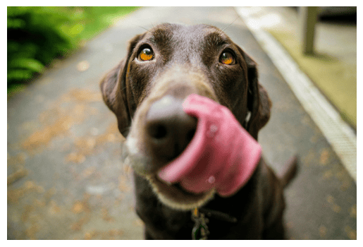
2. Load a query image
3. Define prompts (classifier weights)
4. Compute the embeddings and
5. Zero-shot classification
Apply the classification rule from Section 1:Why raw softmax looks flat
CLIP cosine similarities live in a narrow range. Both encoders produce -normalized embeddings on , and in practice the joint space is a tight cone, so raw dot products typically sit between 0.18 and 0.30 even for good matches. A softmax applied directly to such close values produces a nearly uniform distribution, which makes the classifier look much less confident than it actually is. The fix is the learned temperature parameter that CLIP was trained with (the same that appears in the InfoNCE loss on the CLIP lecture page). In Stable-Baselines3’s HuggingFace wrapper this is stored aslogit_scale = 1/τ ≈ 100. Inference must scale the similarities by before the softmax:
HuggingFace’s CLIP model exposes this scaled value as outputs.logits_per_image, so you get the sharp classification output for free. The cell below compares all three: raw cosine similarity, naive softmax (wrong), temperature-scaled softmax (correct), and the HuggingFace convenience.
6. Visualizing the classifier weights and the image in the same space
Plotting the first 50 components of each text embedding side by side is not very informative, the embeddings live on a -dimensional unit hypersphere and the raw coordinates have no intrinsic meaning. A better view is to project the weights into a low-dimensional subspace and see how they are laid out relative to each other and to the image embedding . Below we fit a 2-component PCA to the text embeddings and project both the text prompts and the image into the same plane. Each labeled point is one classifier weight; the red star is the image embedding . The closest label to the star is the zero-shot prediction .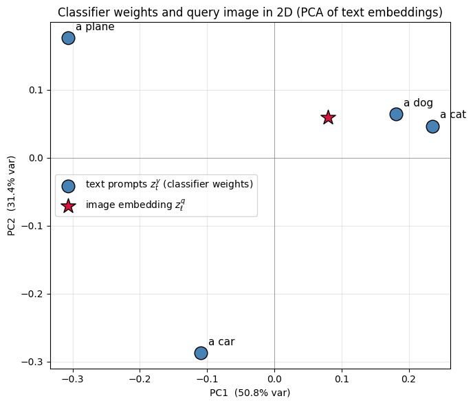
7. Conclusion
We demonstrated that:- Each class prompt produces a vector
- These vectors act as classifier weights
- Zero-shot classification is linear classification in the shared CLIP embedding space
Found an error on this page? Report an issue.