Learning Representations from Pixels

This section was written by Kaushik Kachireddy (pull request #82), with help from an AI coding agent (Claude Code) on the code. It reproduces the ideas of Chapter 30 of Foundations of Computer Vision by Antonio Torralba, Phillip Isola, and William T. Freeman. Representation learning is the forward half of vision: mapping raw pixels to a compact embedding that exposes the underlying factors of a scene. This section builds the book’s demonstrations on its toy colored-shapes dataset:

The dataset (Figure 30.4): 3 shapes by 8 colors, with random size, position, and rotation.
Autoencoders (Figure 30.5): an encoder, a bottleneck, and a decoder. You inspect the embedding through reconstructions, nearest neighbors, and a per-layer probe.
K-means (Figure 30.11): clustering as a discrete representation.
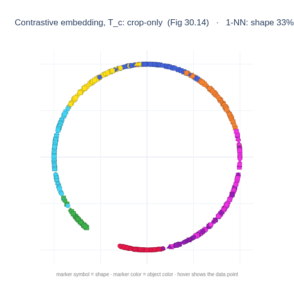
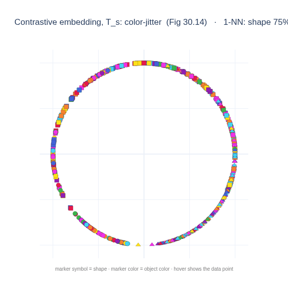
Contrastive learning (Figure 30.14): InfoNCE, where the choice of data augmentation decides whether the embedding encodes color or shape.

The colored-shapes data is procedural in the book too, so it is generated here exactly rather than loaded. Contrastive learning is also the idea behind CLIP, the next section, which applies it across images and text.

import numpy as np, torch, torch.nn as nn, torch.nn.functional as F
import matplotlib.pyplot as plt
import plotly.io as pio
import importlib.util, shutil
if shutil.which('google-chrome') and importlib.util.find_spec('kaleido'):   # a static PNG copy needs kaleido + Chrome
    pio.renderers.default = 'plotly_mimetype+png'   # interactive where supported, plus a static PNG
from PIL import Image, ImageDraw

device = 'cuda' if torch.cuda.is_available() else 'cpu'
_ = torch.manual_seed(0); np.random.seed(0)
torch.set_num_threads(max(1, torch.get_num_threads()))
plt.rcParams.update({'figure.dpi': 130, 'savefig.dpi': 130, 'image.interpolation': 'nearest', 'axes.grid': False})
print('device:', device)

# ---- the toy colored-shapes dataset (Figure 30.4 of the book) ----
COLORS = {'red':(220,50,50),'orange':(240,150,30),'yellow':(235,220,40),'green':(60,180,75),
          'cyan':(40,200,200),'blue':(60,90,220),'purple':(150,60,200),'pink':(240,110,180)}
CNAMES = list(COLORS); SHAPES = ['circle','square','triangle']

def _one(rng, S=32):
    ci, si = rng.integers(8), rng.integers(3)
    base = np.array(COLORS[CNAMES[ci]], float)
    col = tuple(int(np.clip(c + rng.normal(0, 12), 0, 255)) for c in base)   # small color jitter
    img = Image.new('RGB', (S, S), (20, 20, 20)); d = ImageDraw.Draw(img)
    r = rng.integers(int(S*0.22), int(S*0.36))                                # random size
    cx, cy = rng.integers(r, S-r), rng.integers(r, S-r)                        # random position
    ang = rng.uniform(0, 360)                                                  # random rotation
    if si == 0:
        d.ellipse([cx-r, cy-r, cx+r, cy+r], fill=col)
    else:
        n = 4 if si == 1 else 3
        a0 = np.deg2rad(ang) + (np.pi/4 if si == 1 else -np.pi/2)
        pts = [(cx+r*np.cos(a0+2*np.pi*k/n), cy+r*np.sin(a0+2*np.pi*k/n)) for k in range(n)]
        d.polygon(pts, fill=col)
    return np.asarray(img, np.float32)/255.0, si, ci

def make_dataset(n, seed, S=32):
    rng = np.random.default_rng(seed)
    X = np.zeros((n, S, S, 3), np.float32); ys = np.zeros(n, int); yc = np.zeros(n, int)
    for i in range(n): X[i], ys[i], yc[i] = _one(rng, S)
    return X, ys, yc

Xtr, ys_tr, yc_tr = make_dataset(3000, seed=0)
Xte, ys_te, yc_te = make_dataset(600, seed=99)
Xtr_t = torch.tensor(Xtr).permute(0, 3, 1, 2); Xte_t = torch.tensor(Xte).permute(0, 3, 1, 2)
print('train', Xtr.shape, ' test', Xte.shape)

device: cuda

train (3000, 32, 32, 3)  test (600, 32, 32, 3)

The colored-shapes dataset

Each image has one of three shapes (circle, square, triangle) in one of eight colors, with random size, position and rotation. Two independent factors, shape and color, which a representation to disentangle.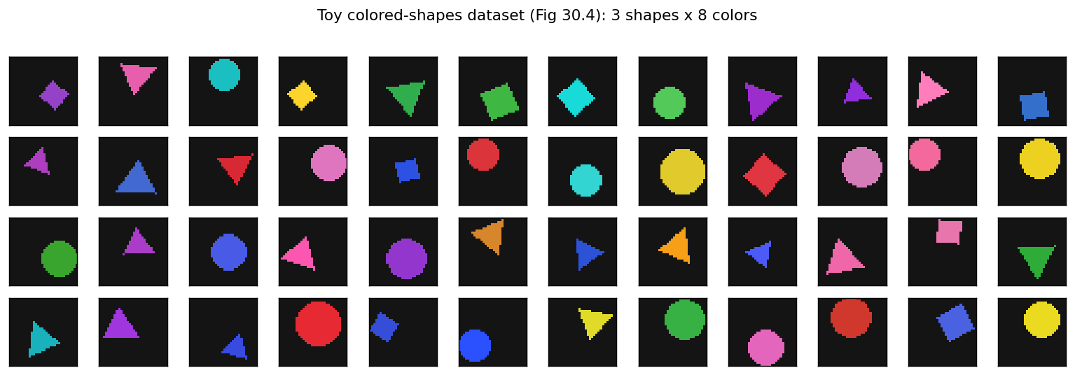

Autoencoders

An autoencoder maps each image through a low-dimensional bottleneck and back, trained to reconstruct its input:

\min_{f,g}\;\mathbb{E}_x\,\lVert g(f(x))-x\rVert^2

. The bottleneck

f(x)

is forced to keep only what is needed to redraw the image, so it becomes a compact representation. You train a small convolutional autoencoder and then look at what its embedding captures.

def cbr(i, o, s): return nn.Sequential(nn.Conv2d(i, o, 3, s, 1), nn.ReLU())
class AE(nn.Module):
    '''The book's autoencoder: six conv layers + a 128-d bottleneck. Downsampling stops
    at 4x4 so deep features keep the spatial detail that distinguishes the shapes.'''
    def __init__(self, M=128):
        super().__init__()
        self.c = nn.ModuleList([cbr(3, 24, 2), cbr(24, 48, 1), cbr(48, 64, 2),
                                cbr(64, 96, 1), cbr(96, 128, 2), cbr(128, 128, 1)])  # 32->16->16->8->8->4->4
        self.bott = nn.Linear(128 * 16, M)
        self.dec = nn.Sequential(nn.Linear(M, 128 * 16), nn.ReLU(), nn.Unflatten(1, (128, 4, 4)),
            nn.ConvTranspose2d(128, 64, 4, 2, 1), nn.ReLU(),
            nn.ConvTranspose2d(64, 32, 4, 2, 1), nn.ReLU(),
            nn.ConvTranspose2d(32, 3, 4, 2, 1), nn.Sigmoid())
    def feats(self, x):                       # input + each of the 6 conv layers (for the probe)
        outs = [x.flatten(1)]; h = x
        for conv in self.c: h = conv(h); outs.append(h.flatten(1))
        return outs
    def encode(self, x):
        h = x
        for conv in self.c: h = conv(h)
        return self.bott(h.flatten(1))        # the 128-d embedding
    def forward(self, x):
        z = self.encode(x); return self.dec(z), z

ae = AE().to(device); opt = torch.optim.Adam(ae.parameters(), 1e-3); lossf = nn.MSELoss()
N = len(Xtr_t)
# The Figure 30.5b crossing needs a real training budget (20k steps): a few minutes on a GPU.
AE_STEPS = 20000
for step in range(AE_STEPS):
    xb = Xtr_t[torch.randint(0, N, (128,))].to(device)
    out, _ = ae(xb); loss = lossf(out, xb)
    opt.zero_grad(); loss.backward(); opt.step()
print(f'autoencoder ({AE_STEPS} steps) trained, reconstruction MSE {loss.item():.4f}')

autoencoder (20000 steps) trained, reconstruction MSE 0.0004

Reconstructions and nearest neighbors

The reconstructions confirm the bottleneck preserves shape, color and rough pose. More interesting: images whose embeddings are nearest neighbors tend to share both shape and color: the embedding has organized the data by its true factors.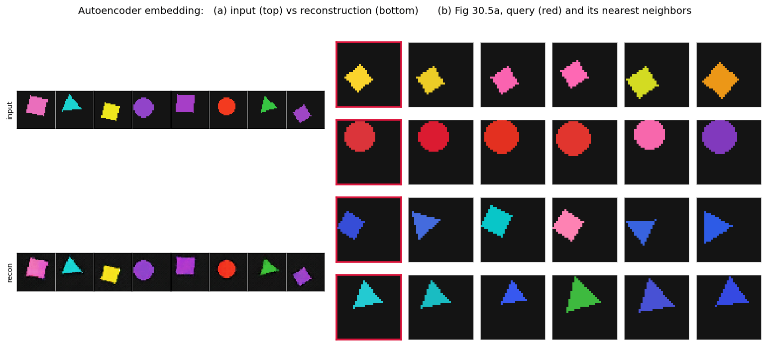

ae.eval()
with torch.no_grad():
    recon, _ = ae(Xte_t[:8].to(device)); recon = recon.cpu()
    Ztr = ae.encode(Xtr_t.to(device)).cpu()
Ztr = F.normalize(Ztr, dim=1)

What does each layer encode?

Probe every layer with a 1-nearest-neighbor classifier (train features -> predict a test image’s shape / color). The two factors are read out very differently across depth: shape accuracy rises toward ~99% in the deeper, more semantic features, while color accuracy falls as the network abstracts away low-level appearance: the crossing the book reports (Fig 30.5b). Reproducing it needs the book’s architecture (six conv layers, keeping spatial detail) and a real training budget; a too-shallow model, or downsampling all the way to a single vector, does not show it.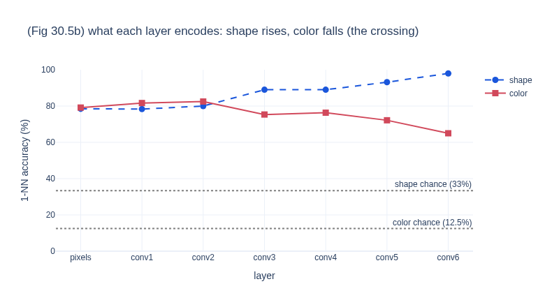

def nn_acc(tr, te, ytr, yte):
    tr = F.normalize(tr, dim=1); te = F.normalize(te, dim=1)
    return (ytr[(te @ tr.T).argmax(1).numpy()] == yte).mean()
# Stream the probe layer-by-layer (forward train+test together, keep only the current
# activations) so we never hold all seven layers' features at once, memory-lean.
ae.eval(); layers = ['pixels', 'conv1', 'conv2', 'conv3', 'conv4', 'conv5', 'conv6']
acc_s, acc_c = [], []
with torch.no_grad():
    htr, hte = Xtr_t.to(device), Xte_t.to(device)
    for i, conv in enumerate([None] + list(ae.c)):
        if conv is not None: htr = conv(htr); hte = conv(hte)
        tr, te = htr.flatten(1).cpu(), hte.flatten(1).cpu()
        acc_s.append(nn_acc(tr, te, ys_tr, ys_te) * 100)
        acc_c.append(nn_acc(tr, te, yc_tr, yc_te) * 100)
        del tr, te

shape: ['78', '78', '80', '89', '89', '93', '98']
color: ['79', '82', '82', '75', '76', '72', '65']

K-means clustering

Clustering yields a discrete representation: each point is summarized by the index of its nearest code vector. K-means minimises

\sum_i \lVert z_{a_i} - x^{(i)}\rVert^2

by block-coordinate descent, alternating: (assign) each point to its nearest mean, (update) each mean to the average of its assigned points. The figure shows the first iterations on a 2-D dataset with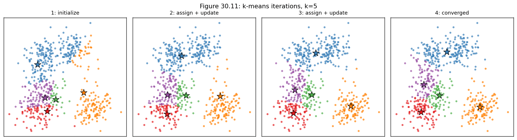

k=5

(Fig 30.11).

g = np.random.default_rng(2)
centers_true = g.uniform(-1, 1, (5, 2)) * 2.2
pts = np.concatenate([c + g.normal(0, 0.45, (120, 2)) for c in centers_true])
k = 5
z = pts[g.choice(len(pts), k, replace=False)].copy()      # init code vectors
palette = np.array(['#e41a1c', '#377eb8', '#4daf4a', '#984ea3', '#ff7f00'])
snaps = []
for it in range(4):
    a = np.argmin(((pts[:, None, :] - z[None]) ** 2).sum(2), axis=1)   # assign
    snaps.append((z.copy(), a.copy()))
    for j in range(k):
        if (a == j).any(): z[j] = pts[a == j].mean(0)                  # update

Contrastive learning: the augmentation chooses the invariance

Contrastive learning pulls together two augmented views of the same image (a positive pair) while pushing apart different images, via the InfoNCE loss:

\mathcal{L} = -\log \frac{e^{f(x)^\top f(x^+)/\tau}}{e^{f(x)^\top f(x^+)/\tau} + \sum_i e^{f(x)^\top f(x_i^-)/\tau}}.

The representation becomes invariant to whatever the augmentation changes. So the choice of augmentation decides which factor survives (embedding dimension

M=2

, so it can be plotted directly on the unit circle):

crop only ( $T_c$ ): keeps color, varies which part of the shape is seen -> the embedding organizes by color;
color jitter ( $T_s$ ): destroys color, keeps shape -> the embedding organizes by shape.

class Enc(nn.Module):
    def __init__(self):
        super().__init__()
        self.net = nn.Sequential(nn.Conv2d(3, 16, 3, 2, 1), nn.ReLU(), nn.Conv2d(16, 32, 3, 2, 1), nn.ReLU(),
            nn.Conv2d(32, 64, 3, 2, 1), nn.ReLU(), nn.Flatten(), nn.Linear(64*16, 64), nn.ReLU(), nn.Linear(64, 2))
    def forward(self, x): return F.normalize(self.net(x), dim=1)      # onto the unit circle

def rand_crop(xb, lo=0.5):
    N, C, H, W = xb.shape; out = torch.empty_like(xb)
    for i in range(N):
        s = float(torch.empty(1).uniform_(lo, 1.0)); ch = max(8, int(H*s)); cw = max(8, int(W*s))
        top = int(torch.randint(0, H-ch+1, (1,))); left = int(torch.randint(0, W-cw+1, (1,)))
        out[i] = F.interpolate(xb[i:i+1, :, top:top+ch, left:left+cw], size=(H, W), mode='bilinear', align_corners=False)[0]
    return out
def color_jitter(xb):
    N = xb.shape[0]; gain = torch.empty(N, 3, 1, 1, device=xb.device).uniform_(0.4, 1.6)
    bright = torch.empty(N, 1, 1, 1, device=xb.device).uniform_(0.6, 1.4)
    perm = torch.stack([torch.randperm(3) for _ in range(N)])
    xj = torch.stack([xb[i, perm[i]] for i in range(N)])
    return (xj * gain * bright).clamp(0, 1)
def small_shift(xb):
    sh = torch.randint(-3, 4, (2,)); return torch.roll(xb, (int(sh[0]), int(sh[1])), dims=(2, 3))

def infonce(z1, z2, tau=0.2):
    z = torch.cat([z1, z2]); sim = z @ z.T / tau; n = len(z1)
    sim.fill_diagonal_(-1e9)
    targets = torch.cat([torch.arange(n) + n, torch.arange(n)]).to(z.device)
    return F.cross_entropy(sim, targets)

def train_contrastive(aug, steps, bs=128, seed=1):
    _ = torch.manual_seed(seed); net = Enc().to(device); opt = torch.optim.Adam(net.parameters(), 1e-3)
    for st in range(steps):
        xb = Xtr_t[torch.randint(0, N, (bs,))].to(device)
        loss = infonce(net(aug(xb)), net(aug(xb))); opt.zero_grad(); loss.backward(); opt.step()
    net.eval()
    with torch.no_grad(): Z = net(Xtr_t.to(device)).cpu().numpy()
    return Z

Z_color = train_contrastive(lambda x: rand_crop(x), steps=1500)               # crop only -> color
Z_shape  = train_contrastive(lambda x: color_jitter(small_shift(x)), steps=2500)  # jitter -> shape
print('trained both contrastive encoders')

trained both contrastive encoders

Summary

A representation re-expresses pixels in terms of their underlying factors. Here the factors are shape and color, and different methods expose them differently.
An autoencoder learns a reusable embedding without labels. Its nearest neighbors respect shape and color, and depth trades low-level appearance (color) for more semantic structure (shape).
K-means is the discrete cousin: a representation by cluster index.
Contrastive learning makes the control explicit: the augmentation you choose is exactly the invariance you get. Crop-only keeps color; color jitter keeps shape. This is the knob behind modern self-supervised encoders, and behind CLIP, where the two views of a pair are an image and its caption.

Edit this page on GitHub or file an issue.

Vision and Language

Representation Learning

Vision-Language Models

VLM SFT Lab

Learning Representations from Pixels

The colored-shapes dataset

Autoencoders

Reconstructions and nearest neighbors

What does each layer encode?

K-means clustering

Contrastive learning: the augmentation chooses the invariance

Summary

​The colored-shapes dataset

​Autoencoders

​Reconstructions and nearest neighbors

​What does each layer encode?

​K-means clustering

​Contrastive learning: the augmentation chooses the invariance

​Summary

The colored-shapes dataset

Autoencoders

Reconstructions and nearest neighbors

What does each layer encode?

K-means clustering

Contrastive learning: the augmentation chooses the invariance

Summary