Open In Colab
title: Using ConvNets with Small Datasets This notebook is a PyTorch adaptation of the canonical small-dataset convnet example from Deep Learning with Python (F. Chollet, Chapter 5). We use the pantelism/cats-vs-dogs dataset hosted on Hugging Face (the same 4,000-image Kaggle subset used in the original) and demonstrate:
  1. Baseline: training a small convnet from scratch → clear overfitting with only 2,000 training samples
  2. Regularization: data augmentation + dropout → substantially lower validation loss and higher accuracy
The trained model is saved as cats_and_dogs_small.pth for use by the companion visualization notebook.
!pip install datasets scikit-learn seaborn --quiet
import numpy as np
import matplotlib.pyplot as plt
import torch
import torch.nn as nn
from torch.utils.data import DataLoader
from torchvision import transforms
from sklearn.metrics import confusion_matrix, roc_curve
import seaborn as sns

# ── Config ──────────────────────────────────────────────────────────────────
IMG_SIZE        = 150
BATCH_SIZE      = 32
EPOCHS_BASELINE = 20   # enough to show overfitting clearly
EPOCHS_AUG      = 30   # enough to show regularisation benefit
LR              = 1e-4
SEED            = 42

DEVICE = torch.device("cuda" if torch.cuda.is_available() else "cpu")
print(f"Device: {DEVICE}")
Device: cuda

Dataset

pantelism/cats-vs-dogs is a Parquet imagefolder dataset on Hugging Face containing the 4,000-image Kaggle cats-vs-dogs subset used in the original Chollet notebook. It has three pre-built splits — train (2,000 images), validation (1,000), and test (1,000) — with a ClassLabel feature mapping 0 → cat and 1 → dog. We load it directly with load_dataset and wrap it in a lightweight PyTorch Dataset.
from datasets import load_dataset
from torch.utils.data import Dataset

# ── Load dataset ──────────────────────────────────────────────────────────────
# pantelism/cats-vs-dogs is a Parquet imagefolder dataset with three splits
ds_dict = load_dataset("pantelism/cats-vs-dogs")

label_names = ds_dict["train"].features["label"].names  # ['cat', 'dog']
print(f"Train {len(ds_dict['train'])} | Val {len(ds_dict['validation'])} | Test {len(ds_dict['test'])}")
print("Labels:", label_names)

# ── PyTorch Dataset wrapper ───────────────────────────────────────────────────
class CatsDogsDataset(Dataset):
    def __init__(self, hf_dataset, transform):
        self.data      = hf_dataset
        self.transform = transform

    def __len__(self):
        return len(self.data)

    def __getitem__(self, idx):
        sample = self.data[idx]
        img    = sample["image"].convert("RGB")
        label  = float(sample["label"])   # ClassLabel int → float for BCEWithLogitsLoss
        return self.transform(img), label

# ── Transforms ───────────────────────────────────────────────────────────────
basic_tf = transforms.Compose([
    transforms.Resize((IMG_SIZE, IMG_SIZE)),
    transforms.ToTensor(),
    transforms.Normalize([0.5, 0.5, 0.5], [0.5, 0.5, 0.5]),
])

aug_tf = transforms.Compose([
    transforms.Resize((IMG_SIZE, IMG_SIZE)),
    transforms.RandomHorizontalFlip(),
    transforms.RandomRotation(40),
    transforms.RandomAffine(degrees=0, translate=(0.2, 0.2), shear=20),
    transforms.RandomResizedCrop(IMG_SIZE, scale=(0.8, 1.0)),
    transforms.ColorJitter(brightness=0.1, contrast=0.1),
    transforms.ToTensor(),
    transforms.Normalize([0.5, 0.5, 0.5], [0.5, 0.5, 0.5]),
])

# ── DataLoaders ──────────────────────────────────────────────────────────────
def make_loader(hf_split, tf, shuffle=False):
    return DataLoader(
        CatsDogsDataset(hf_split, tf),
        batch_size=BATCH_SIZE,
        shuffle=shuffle,
        num_workers=2,
        pin_memory=True,
    )

train_loader_basic = make_loader(ds_dict["train"],      basic_tf, shuffle=True)
train_loader_aug   = make_loader(ds_dict["train"],      aug_tf,   shuffle=True)
val_loader         = make_loader(ds_dict["validation"], basic_tf)
test_loader        = make_loader(ds_dict["test"],       basic_tf)

imgs, labels = next(iter(train_loader_basic))
print(f"Batch shape: {imgs.shape}, Labels: {labels[:8].tolist()}")
Train 2000 | Val 1000 | Test 1000
Labels: ['cat', 'dog']
Batch shape: torch.Size([32, 3, 150, 150]), Labels: [0.0, 1.0, 0.0, 0.0, 1.0, 0.0, 1.0, 0.0]

Model architecture

We replicate the Chollet convnet — four Conv2d → ReLU → MaxPool2d blocks that progressively increase depth (32 → 64 → 128 → 128) while halving spatial dimensions (150 → 74 → 36 → 17 → 7), followed by a fully-connected head. An optional Dropout(0.5) layer is inserted before the first dense layer for the regularised variant.
Input 3×150×150
  Conv2d(3→32, k=3)  → ReLU → MaxPool2d(2)   →  32×74×74
  Conv2d(32→64, k=3) → ReLU → MaxPool2d(2)   →  64×36×36
  Conv2d(64→128,k=3) → ReLU → MaxPool2d(2)   → 128×17×17
  Conv2d(128→128,k=3)→ ReLU → MaxPool2d(2)   → 128×7×7
  Flatten → [Dropout(0.5)] → Linear(6272→512) → ReLU → Linear(512→1)
class SmallConvNet(nn.Module):
    def __init__(self, dropout: bool = False):
        super().__init__()
        self.features = nn.Sequential(
            nn.Conv2d(3,   32,  3), nn.ReLU(), nn.MaxPool2d(2),
            nn.Conv2d(32,  64,  3), nn.ReLU(), nn.MaxPool2d(2),
            nn.Conv2d(64,  128, 3), nn.ReLU(), nn.MaxPool2d(2),
            nn.Conv2d(128, 128, 3), nn.ReLU(), nn.MaxPool2d(2),
        )
        self.classifier = nn.Sequential(
            nn.Dropout(0.5) if dropout else nn.Identity(),
            nn.Linear(128 * 7 * 7, 512),
            nn.ReLU(),
            nn.Linear(512, 1),
        )

    def forward(self, x: torch.Tensor) -> torch.Tensor:
        x = self.features(x)
        x = x.view(x.size(0), -1)
        return self.classifier(x).squeeze(1)   # shape (B,)

# Verify output shape
_dummy = torch.zeros(2, 3, IMG_SIZE, IMG_SIZE)
assert SmallConvNet()(_dummy).shape == (2,), "unexpected output shape"
print("Architecture verified — output shape (B,) ✓")
print(SmallConvNet())
Architecture verified — output shape (B,) ✓
SmallConvNet(
  (features): Sequential(
    (0): Conv2d(3, 32, kernel_size=(3, 3), stride=(1, 1))
    (1): ReLU()
    (2): MaxPool2d(kernel_size=2, stride=2, padding=0, dilation=1, ceil_mode=False)
    (3): Conv2d(32, 64, kernel_size=(3, 3), stride=(1, 1))
    (4): ReLU()
    (5): MaxPool2d(kernel_size=2, stride=2, padding=0, dilation=1, ceil_mode=False)
    (6): Conv2d(64, 128, kernel_size=(3, 3), stride=(1, 1))
    (7): ReLU()
    (8): MaxPool2d(kernel_size=2, stride=2, padding=0, dilation=1, ceil_mode=False)
    (9): Conv2d(128, 128, kernel_size=(3, 3), stride=(1, 1))
    (10): ReLU()
    (11): MaxPool2d(kernel_size=2, stride=2, padding=0, dilation=1, ceil_mode=False)
  )
  (classifier): Sequential(
    (0): Identity()
    (1): Linear(in_features=6272, out_features=512, bias=True)
    (2): ReLU()
    (3): Linear(in_features=512, out_features=1, bias=True)
  )
)

Baseline: training from scratch with no regularisation

We train for 20 epochs with RMSprop and binary cross-entropy loss. With only 2,000 training samples the network overfits quickly: training accuracy climbs to ~95% while validation accuracy plateaus around 70–72%, a textbook overfitting signature.
def train_model(model, train_loader, val_loader, epochs, lr=LR):
    model = model.to(DEVICE)
    criterion = nn.BCEWithLogitsLoss()
    optimiser = torch.optim.RMSprop(model.parameters(), lr=lr)

    history = dict(train_loss=[], val_loss=[], train_acc=[], val_acc=[])

    for epoch in range(epochs):
        # ── Training pass ────────────────────────────────────────────────────
        model.train()
        t_loss = t_correct = t_n = 0
        for imgs, labels in train_loader:
            imgs   = imgs.to(DEVICE)
            labels = labels.to(DEVICE)   # already float from CatsDogsDataset
            optimiser.zero_grad()
            logits = model(imgs)
            loss   = criterion(logits, labels)
            loss.backward()
            optimiser.step()
            t_loss    += loss.item() * len(imgs)
            t_correct += ((logits > 0) == labels.bool()).sum().item()
            t_n       += len(imgs)

        # ── Validation pass ──────────────────────────────────────────────────
        model.eval()
        v_loss = v_correct = v_n = 0
        with torch.no_grad():
            for imgs, labels in val_loader:
                imgs   = imgs.to(DEVICE)
                labels = labels.float().to(DEVICE)
                logits = model(imgs)
                v_loss    += criterion(logits, labels).item() * len(imgs)
                v_correct += ((logits > 0) == labels.bool()).sum().item()
                v_n       += len(imgs)

        history["train_loss"].append(t_loss / t_n)
        history["train_acc"].append(t_correct / t_n)
        history["val_loss"].append(v_loss / v_n)
        history["val_acc"].append(v_correct / v_n)

        if (epoch + 1) % 5 == 0 or epoch == 0:
            print(
                f"Epoch {epoch+1:3d}/{epochs}  "
                f"loss {history['train_loss'][-1]:.4f}  acc {history['train_acc'][-1]:.3f}  |  "
                f"val_loss {history['val_loss'][-1]:.4f}  val_acc {history['val_acc'][-1]:.3f}"
            )
    return history


def plot_history(history, title, save_path=None):
    epochs = range(1, len(history["train_acc"]) + 1)
    fig, (ax1, ax2) = plt.subplots(1, 2, figsize=(12, 4))
    ax1.plot(epochs, history["train_acc"], "bo-", label="Training")
    ax1.plot(epochs, history["val_acc"],   "b-",  label="Validation")
    ax1.set_title(f"{title} — Accuracy"); ax1.set_xlabel("Epoch"); ax1.legend()
    ax2.plot(epochs, history["train_loss"], "ro-", label="Training")
    ax2.plot(epochs, history["val_loss"],   "r-",  label="Validation")
    ax2.set_title(f"{title} — Loss"); ax2.set_xlabel("Epoch"); ax2.legend()
    plt.tight_layout()
    if save_path:
        plt.savefig(save_path, dpi=120, bbox_inches="tight")
    plt.show()


torch.manual_seed(SEED)
model_baseline = SmallConvNet(dropout=False)
print("Training baseline …")
hist_baseline = train_model(model_baseline, train_loader_basic, val_loader, EPOCHS_BASELINE)
plot_history(hist_baseline, "Baseline (no augmentation)", "baseline_curves.png")
Training baseline …
Epoch   1/20  loss 0.6910  acc 0.535  |  val_loss 0.7333  val_acc 0.500
Epoch   5/20  loss 0.5520  acc 0.719  |  val_loss 0.6378  val_acc 0.646
Epoch  10/20  loss 0.4618  acc 0.797  |  val_loss 0.5756  val_acc 0.714
Epoch  15/20  loss 0.3708  acc 0.837  |  val_loss 0.6378  val_acc 0.699
Epoch  20/20  loss 0.2830  acc 0.885  |  val_loss 0.5921  val_acc 0.733
Baseline training curves — accuracy and loss showing overfitting after epoch 5

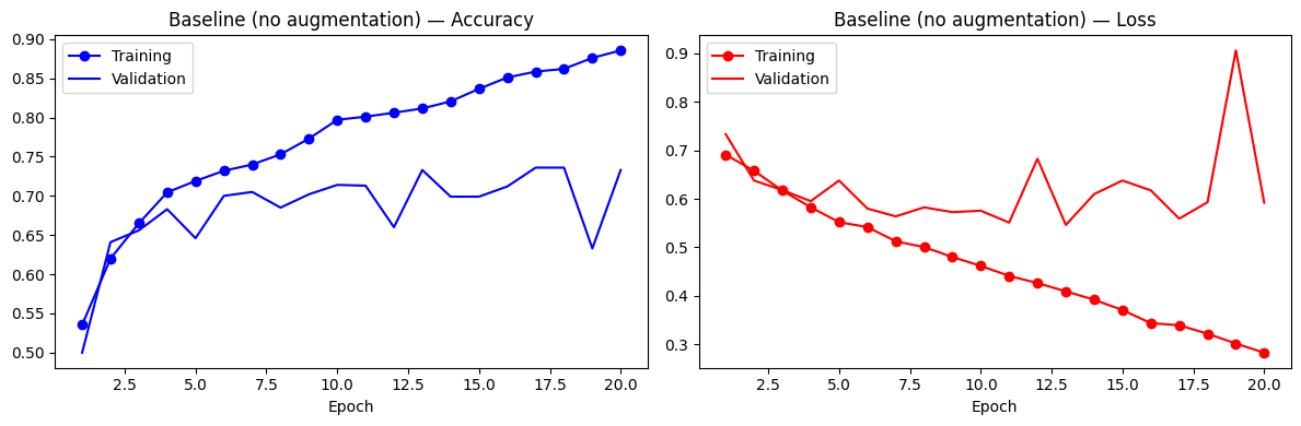
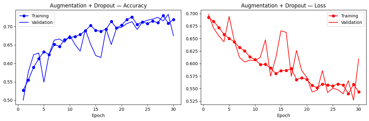
Data augmentation + dropout

Data augmentation generates new views of each training image on-the-fly — random horizontal flips, rotations, translations, shears, and crop-resizes — so the model never sees the exact same pixel pattern twice. Combined with Dropout(0.5), this substantially reduces the train-validation gap characteristic of overfitting.
torch.manual_seed(SEED)
model_aug = SmallConvNet(dropout=True)
print("Training augmented model (data augmentation + dropout) …")
hist_aug = train_model(model_aug, train_loader_aug, val_loader, EPOCHS_AUG)
plot_history(hist_aug, "Augmentation + Dropout", "augmented_curves.png")
Training augmented model (data augmentation + dropout) …
Epoch   1/30  loss 0.6924  acc 0.527  |  val_loss 0.6984  val_acc 0.500
Epoch   5/30  loss 0.6503  acc 0.631  |  val_loss 0.6941  val_acc 0.549
Epoch  10/30  loss 0.6079  acc 0.670  |  val_loss 0.6061  val_acc 0.676
Epoch  15/30  loss 0.5857  acc 0.690  |  val_loss 0.6656  val_acc 0.621
Epoch  20/30  loss 0.5683  acc 0.704  |  val_loss 0.5722  val_acc 0.698
Epoch  25/30  loss 0.5554  acc 0.708  |  val_loss 0.5508  val_acc 0.717
Epoch  30/30  loss 0.5436  acc 0.719  |  val_loss 0.6092  val_acc 0.675
Augmented model training curves — tighter train/validation gap from data augmentation and dropout

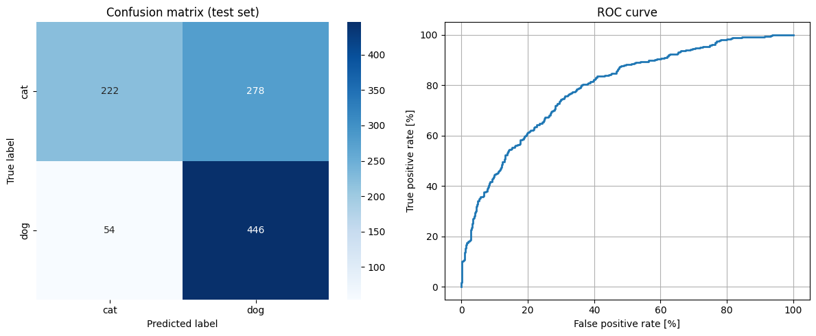
Evaluation on the held-out test set

We evaluate the regularised model on the 1,000-image test split and report:
  • Confusion matrix — to see which mistakes are made
  • ROC curve — to characterise the trade-off across thresholds
  • Test accuracy — headline metric
The model is saved as cats_and_dogs_small.pth for the companion visualisation notebook.
# ── Save model ───────────────────────────────────────────────────────────────
torch.save(model_aug.state_dict(), "cats_and_dogs_small.pth")
print("Saved cats_and_dogs_small.pth")

# ── Collect predictions ──────────────────────────────────────────────────────
model_aug.eval()
all_labels, all_probs = [], []
with torch.no_grad():
    for imgs, labels in test_loader:
        logits = model_aug(imgs.to(DEVICE))
        probs  = torch.sigmoid(logits).cpu().numpy()
        all_probs.extend(probs)
        all_labels.extend(labels.numpy())

all_labels = np.array(all_labels, dtype=int)
all_probs  = np.array(all_probs)
preds      = (all_probs > 0.5).astype(int)

# ── Confusion matrix + ROC ───────────────────────────────────────────────────
fig, axes = plt.subplots(1, 2, figsize=(12, 5))

cm = confusion_matrix(all_labels, preds)
sns.heatmap(cm, annot=True, fmt="d", ax=axes[0], cmap="Blues",
            xticklabels=label_names, yticklabels=label_names)
axes[0].set_title("Confusion matrix (test set)")
axes[0].set_ylabel("True label"); axes[0].set_xlabel("Predicted label")

fp, tp, _ = roc_curve(all_labels, all_probs)
axes[1].plot(100 * fp, 100 * tp, linewidth=2)
axes[1].set_xlabel("False positive rate [%]"); axes[1].set_ylabel("True positive rate [%]")
axes[1].set_title("ROC curve"); axes[1].grid(True)

plt.tight_layout()
plt.savefig("evaluation.png", dpi=120, bbox_inches="tight")
plt.show()

acc = (preds == all_labels).mean()
print(f"Test accuracy: {acc:.3f}")
Saved cats_and_dogs_small.pth
Confusion matrix and ROC curve on the held-out test set
Test accuracy: 0.668