Feature Extraction via Residual Networks
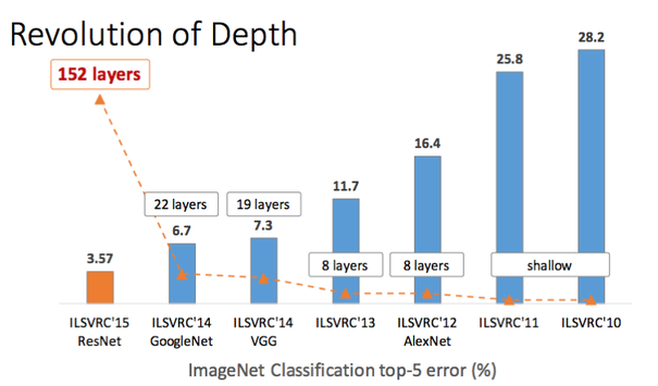
In the figure below we plot the evolution of depth in CNN architectures. Notice the big jump due to the introduction of the ResNet architecture.
 Evolution of depth in CNN architectures. (Circa 2018)
The aim of this section is to provide an alternative view as to why ResNets seem to be able to accommodate much deeper architecture while performing even better that existing architectures for the same depth (e.g. ResNet-18).
The ResNet Architecture
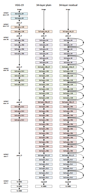
 34 layers deep ResNet architecture (3rd column) vs earlier architectures
ResNets or residual networks, introduced the concept of the residual. This can be understood looking at a small residual network of three stages. The striking difference between ResNets and earlier architectures are the skip connections. Shortcut connections are those skipping one or more layers. The shortcut connections simply perform identity mapping, and their outputs are added to the outputs of the stacked layers. Identity shortcut connections add neither extra parameter nor computational complexity. The entire network can still be trained end-to-end by SGD with backpropagation, and can be easily implemented using common libraries without modifying the solvers.
Hinton showed that dropping out individual neurons during training leads to a network that is equivalent to averaging over an ensemble of exponentially many networks. Entire layers can be removed from plain residual networks without impacting performance, indicating that they do not strongly depend on each other.
Each layer consists of a residual module \(f_i\) and a skip connection bypassing \(f_i\). Since layers in residual networks can comprise multiple convolutional layers, we refer to them as residual blocks. With \(y_{i-1}\) as is input, the output of the i-th block is recursively defined as
\(y_i = f_i(y_{i−1}) + y_{i−1}\)
where \(f_i(x)\) is some sequence of convolutions, batch normalization, and Rectified Linear Units (ReLU) as nonlinearities. In the figure above we have three blocks. Each \(f_i(x)\) is defined by
\(f_i(x) = W_i^{(1)} * \sigma(B (W_i^{(2)} * \sigma(B(x))))\)
where \(W_i^{(1)}\) and \(W_i^{(2)}\) are weight matrices, · denotes convolution, \(B(x)\) is batch normalization and \(\sigma(x) ≡ max(x, 0)\). Other formulations are typically composed of the same operations, but may differ in their order.
During the lecture we will go through this paper analysis of the unrolled network to understand the behavior of ResNets that are inherently scalable networks.
ResNets are commonly used as feature extractors for object detection as in this tutorial.
These networks are the obvious / typical choice today and they can also be used in real time video streaming applications achieving significant frames per second throughputs.
ResNets and Batch Normalization
This notebook is very instructive of what now is considered a canonical new ResNet block that includes batch normalization.
