Convolutional Layer
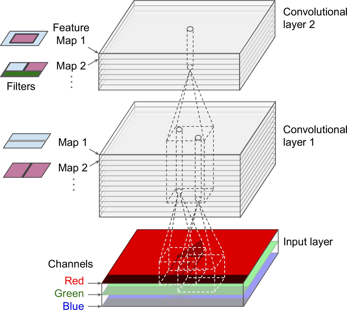
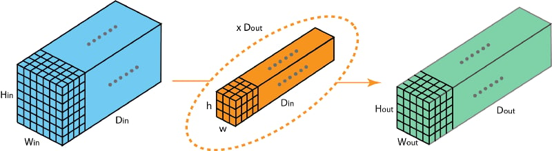
In the convolutional layer the first operation a 3D image with its two spatial dimensions and its third dimension due to the primary colors, typically Red Green and Blue is at the input layer, is convolved with a 3D structure called the filter shown below.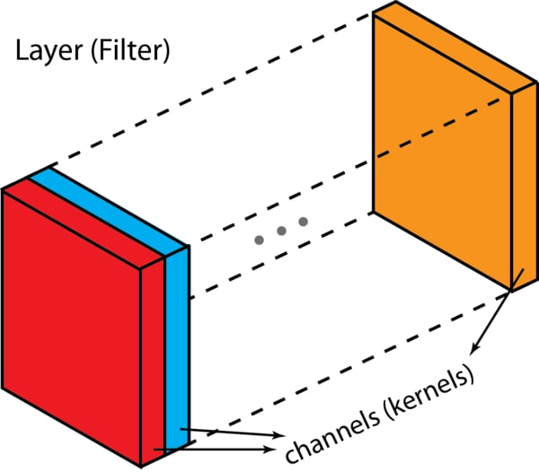
You may need to click on animated example to see the animation depedning on the size of your screen.
Zero Padding
Few words about padding. There are two types:samepadding: output size is the same as input size when stride is 1. This requires the filter window to slip outside input map, hence the need to pad.validpadding: filter stays at valid position inside the input map, so output size shrinks by filter_size - 1. No padding occurs.
Dilation
Dilation (atrous rate) is spacing between kernel taps.d=1: normal conv (adjacent kernel elements).d>1: inserts gaps, so the kernel covers a larger area without increasing parameter count much.
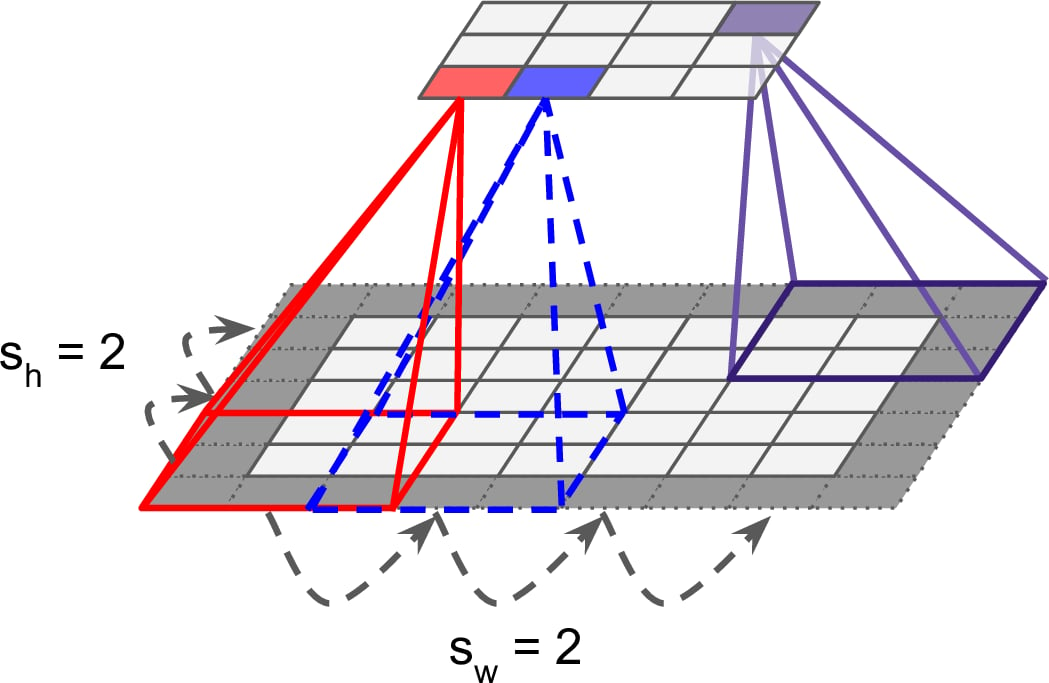
Output size calculation
in: input sizek: kernel sizes: stridep: paddingd: dilation
same padding (p=1) and stride 1, the output feature map has the same spatial dimensions as the input feature map.
What the convolution / operation offers
There are two main consequences of the convolution operation: sparsity and parameter sharing. With the later we get as a byproduct equivariance to translation. These are explained next.Sparsity
In DNNs, every output unit interacts with every input unit. Convolutional networks, however, typically have sparse interactions(also referred to as sparse connectivity or sparse weights). This is accomplished by making the kernel smaller than the input as shown in the figure above. For example,when processing an image, the input image might have thousands or millions of pixels, but we can detect small, meaningful features such as edges with kernels that have much smaller receptive fields.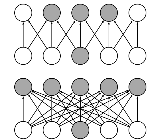
Parameter sharing
In CNNs, each member of the kernel is used at every feasible position of the input. The parameter sharing used by the convolution operation means that rather than learning a separate set of parameters for every location, we learn only one set.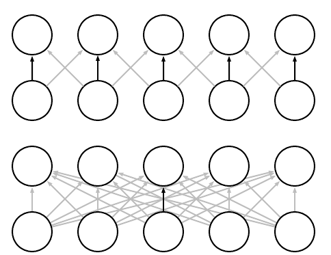
Pooling
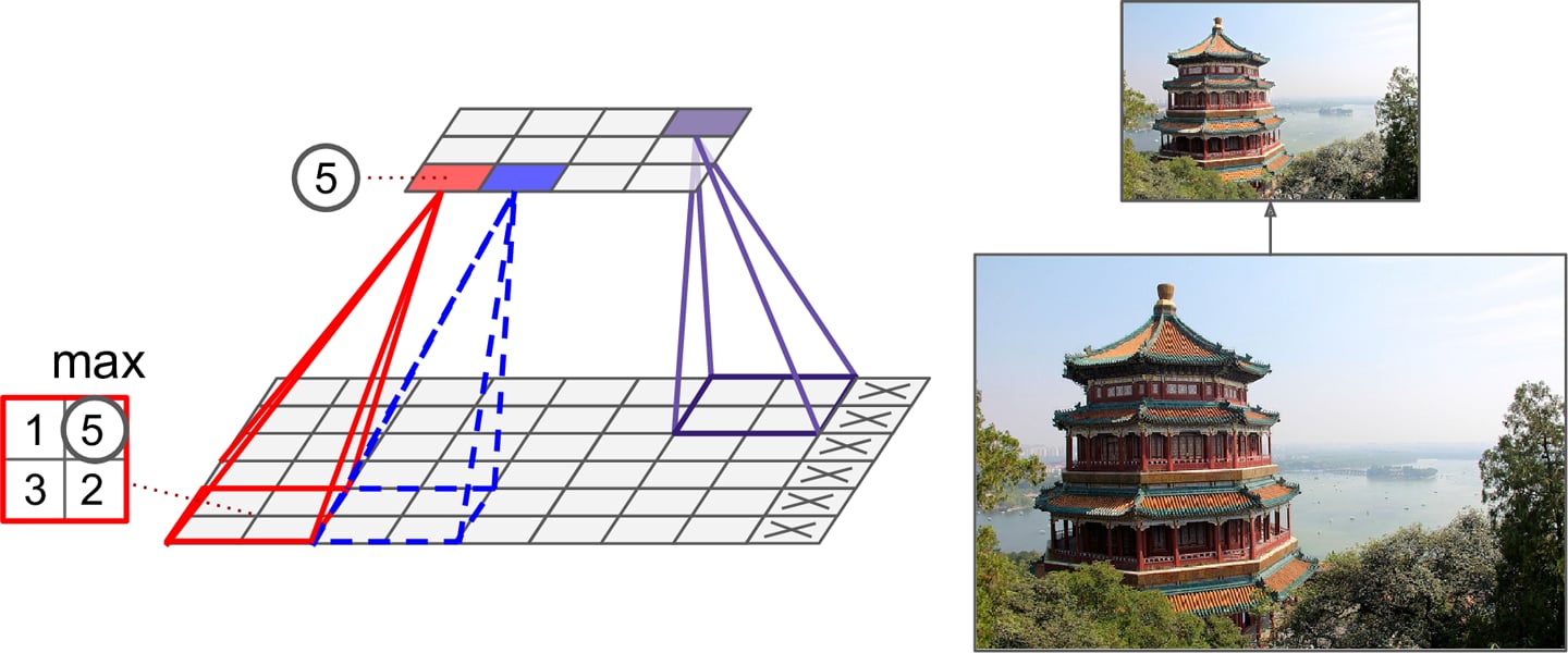
Pooling was introduced to reduce redundancy of representation and reduce the number of parameters, recognizing that precise location is not important for object detection. The pooling function is a form of non-linear function that further modifies the result of the RELU result. The pooling function accepts as input pixel values surrounding (a rectangular region) a feature map location (i,j) and returns one of the following- the maximum,
- the average or distance weighted average,
- the L2 norm.
- Datasets are so big that we’re more concerned about under-fitting.
- Dropout is a much better regularizer.
- Pooling results in a loss of information - think about the max-pooling operation as an example shown in the figure below.
- All convolutional networks where the pooling is replaced by a CNN with larger stride can do better.
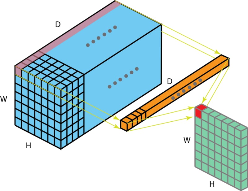
1x1 Convolutional layer
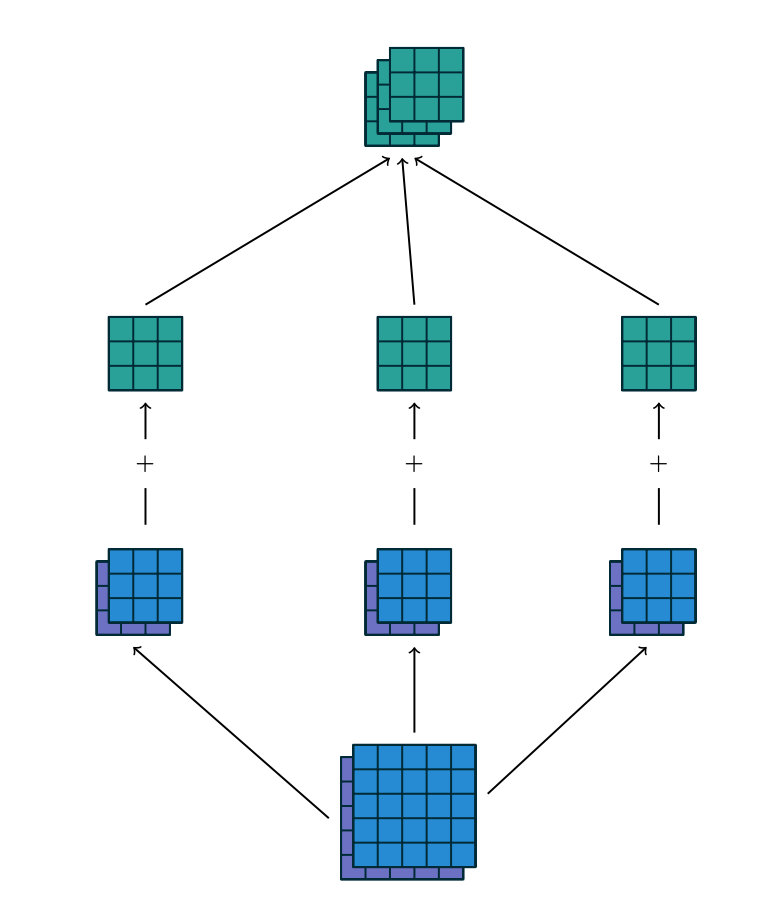
The 1x1 convolution layer is met in many network architectures (e.g. GoogleNet) and offers a number of modeling capabilities. Spatially, the 1x1 convolution is equivalent to a single number multiplication of each spatial position of the input feature map (if we ignore the non-linearity) as shown below. This means that leaves the spatial dimensions of the input feature maps unchanged unlike the pooling layer.
PyTorch reference
| PyTorch class | Description |
|---|---|
nn.Conv2d | Applies a 2D convolution over an input signal composed of several input planes. |
nn.ReLU | Applies the rectified linear unit function element-wise. |
nn.MaxPool2d | Applies a 2D max pooling over an input signal composed of several input planes. |
nn.AvgPool2d | Applies a 2D average pooling over an input signal composed of several input planes. |
References
- Dumoulin, V., Visin, F. (2016). A guide to convolution arithmetic for deep learning.
- Howard, A., Zhu, M., Chen, B., Kalenichenko, D., Wang, W., et al. (2017). MobileNets: Efficient Convolutional Neural Networks for Mobile Vision Applications.
- Peng, X., Sun, B., Ali, K., Saenko, K. (2015). What Do Deep CNNs Learn About Objects?.
- Simonyan, K., Zisserman, A. (2014). Very Deep Convolutional Networks for Large-Scale Image Recognition.
- Zeiler, M., Fergus, R. (2013). Visualizing and Understanding Convolutional Networks.