Neuron
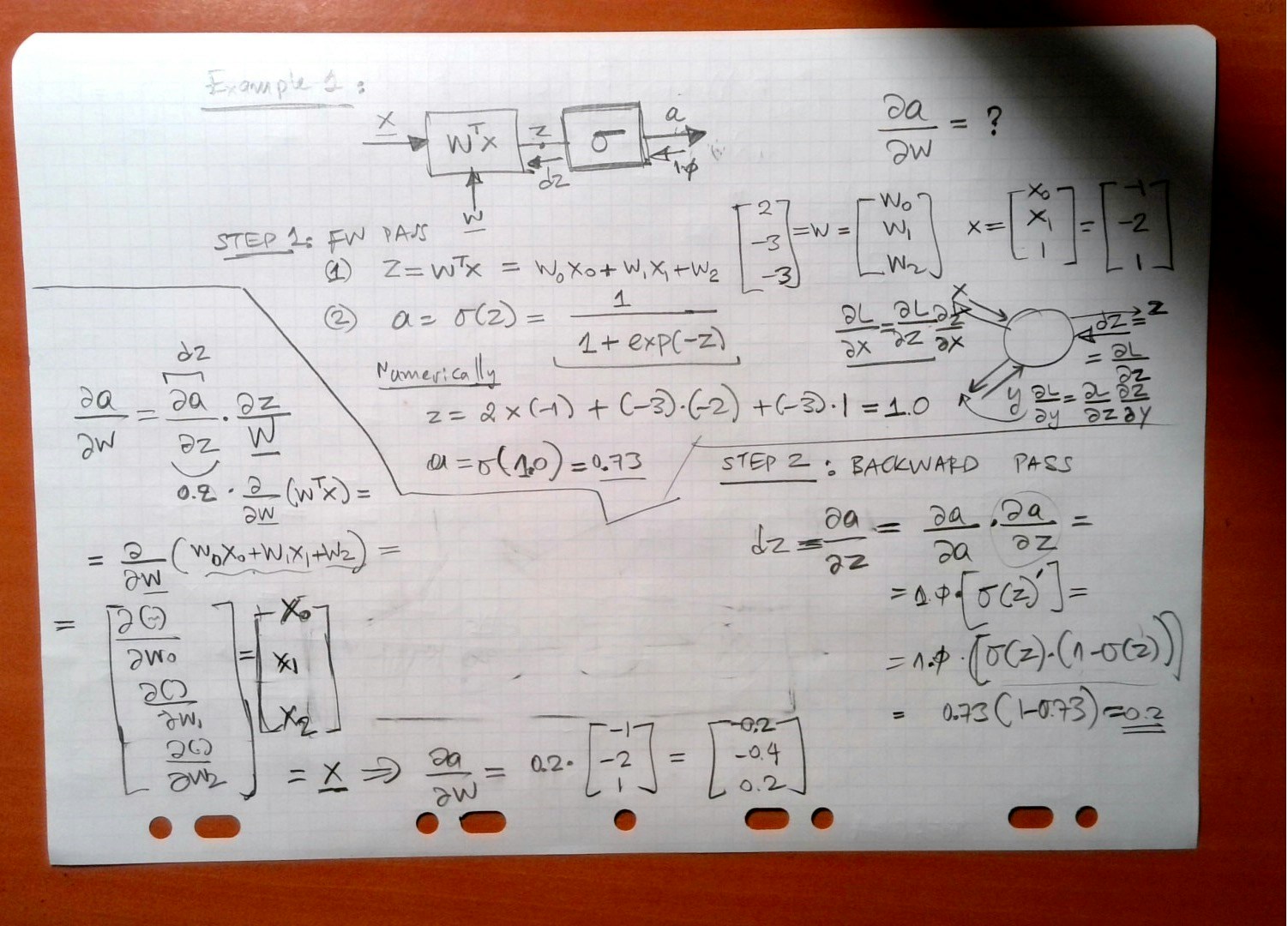
Simple DNN 1
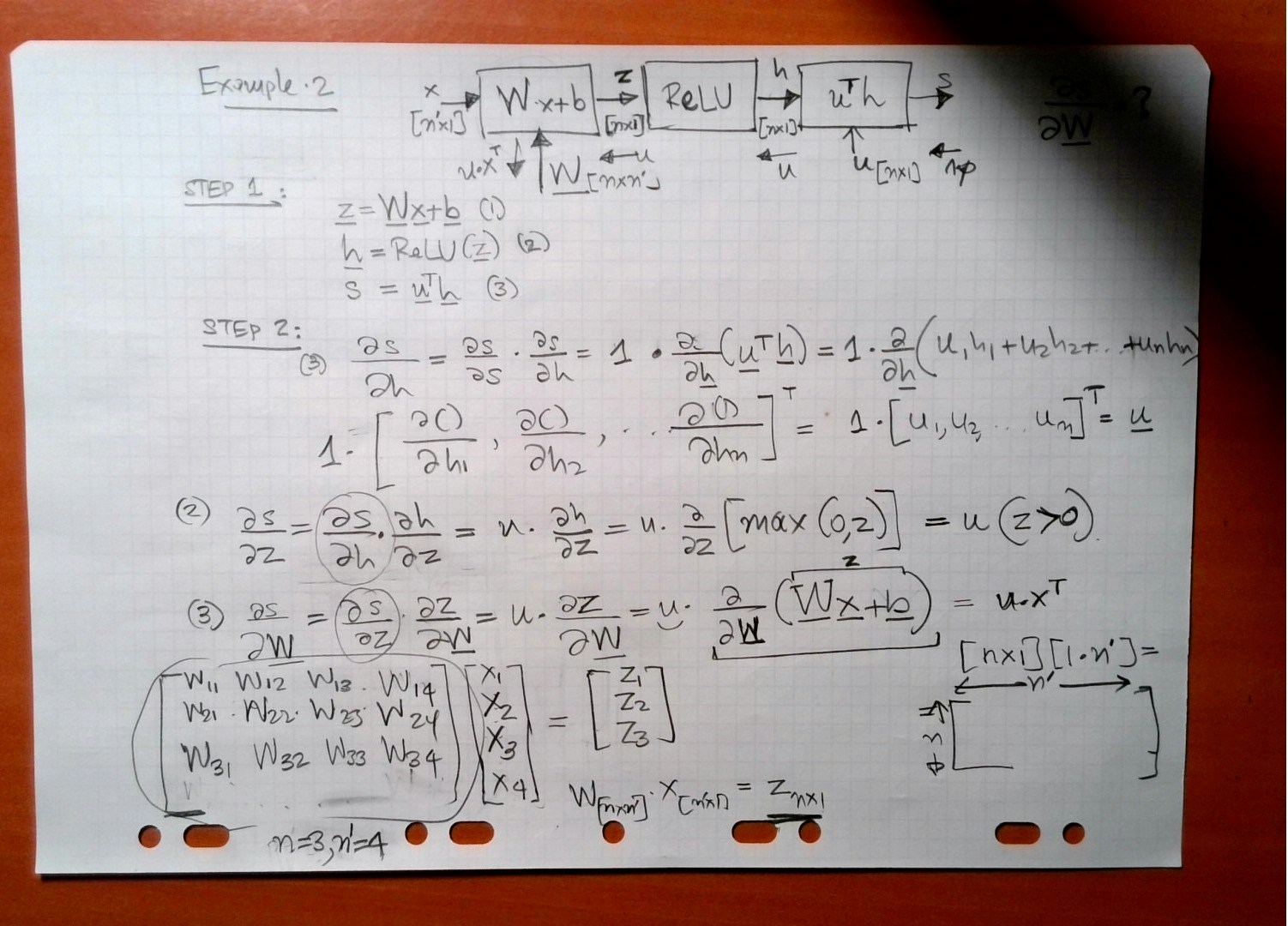
Simple DNN 2
A network consist of a concatenation of the following layers- Fully Connected layer with input , and output .
- RELU producing
- Fully Connected layer with parameters producing
- SOFTMAX producing
- Cross-Entropy (CE) loss producing
- Sketch the network and write down the equations for the forward path.
- Propagate the backwards path i.e. make sure you write down the expressions of the gradient of the loss with respect to all the network parameters.
| Forward Pass Step | Symbolic Equation |
|---|---|
| (1) | |
| (2) | |
| (3) | |
| (4) | |
| (5) |
| Backward Pass Step | Symbolic Equation |
|---|---|
| (5) | |
| (4) | |
| (3a) | |
| (3b) | |
| (2) | if |
| (1) |
References
- Bengio, Y. (2012). Practical recommendations for gradient-based training of deep architectures.
- Bengio, E., Bacon, P., Pineau, J., Precup, D. (2015). Conditional Computation in Neural Networks for faster models.
- Choromanska, A., Henaff, M., Mathieu, M., Ben Arous, G., LeCun, Y. (2014). The Loss Surfaces of Multilayer Networks.
- Jaderberg, M., Czarnecki, W., Osindero, S., Vinyals, O., Graves, A., et al. (2016). Decoupled Neural Interfaces using Synthetic Gradients.
- Romero, A., Ballas, N., Kahou, S., Chassang, A., Gatta, C., et al. (2014). FitNets: Hints for Thin Deep Nets.