In case you have forgotten the basics of calculus, please review the calculus section before proceeding.
Calculating the Gradient of a Function
Our goal is to compute the components of the gradient of the function where, The computational graph of this function is shown below. Its instructive to print this graph and pencil in all calculations for both this example and others in the backpropagation section. One derivative that we will be using that is not often listed is the derivative of the sigmoid function. The sigmoid derivative can be obtained as follows: Consider Then, on the one hand, the chain rule gives and on the other hand, Equating the two expressions we finally obtain,
Forward Pass
In the forward pass, the algorithm works bottom up (or left to right depending how the computational graph is represented) and calculates the values of all “gates” (gates are the elementary functions that synthesize the function) of the graph and stores their values into variables as they will be used by the backwards pass. There are eight values stored in this specific example.Backwards Pass
In the backwards pass, we reverse direction and start at the top or rightmost node (the stored variables) of the graph and compute the input (in the reverse direction) derivative of input of each gate using the template depicted below: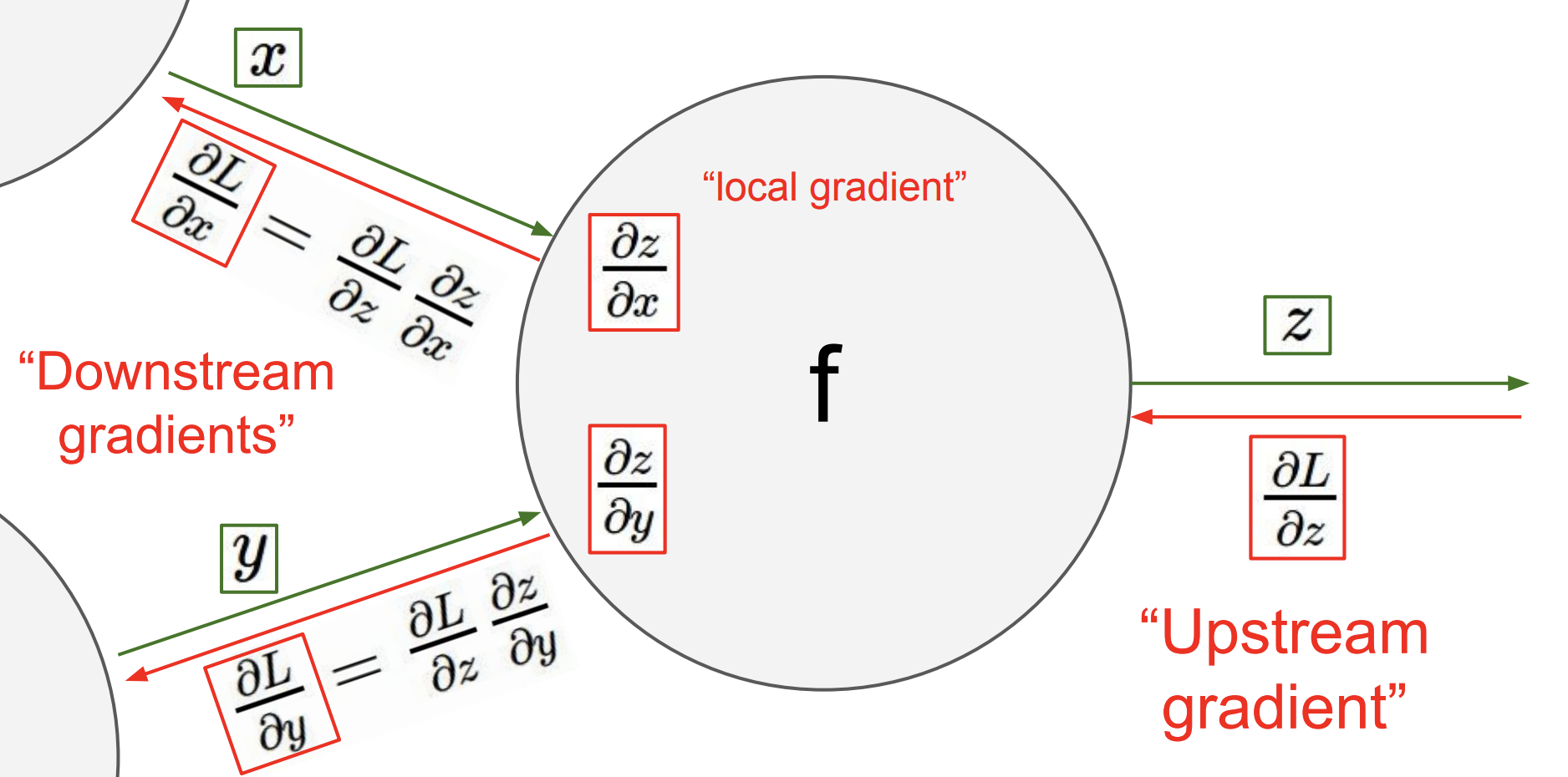
| Gate | Description |
|---|---|
| Add | This gate always takes the gradient on its output and distributes it equally to all of its inputs, regardless of what their values were during the forward pass. This follows from the fact that the local gradient for the add operation is simply +1.0, so the gradients on all inputs will exactly equal the gradients on the output because it will be multiplied by x1.0 (and remain unchanged). |
| Multiply | Its local gradients are the input values (except switched), and this is multiplied by the gradient on its output during the chain rule. Notice that if one of the inputs to the multiply gate is very small and the other is very big, then the multiply gate will do something slightly non intuitive: it will assign a relatively huge gradient to the small input and a tiny gradient to the large input. Note that in linear classifiers where the weights are dot produced (multiplied) with the inputs, this implies that the scale of the data has an effect on the magnitude of the gradient for the weights. For example, if you multiplied all input data examples by 1000 during preprocessing, then the gradient on the weights will be 1000 times larger, and you’d have to lower the learning rate by that factor to compensate. This is why preprocessing matters a lot. |
| Branch (or split) | This gate takes a single input and produces a number of identical copies at the output. With , backpropagating the gate will produce, . This gate was met in the example above and applied in lines were we have dx+= and dy+= expressions. To understand why that is, consider the general form of multivariate chain rule and make sure you also understand its intuition. |
References
- Bengio, Y. (2012). Practical recommendations for gradient-based training of deep architectures.
- Choromanska, A., Henaff, M., Mathieu, M., Ben Arous, G., LeCun, Y. (2014). The Loss Surfaces of Multilayer Networks.
- Lin, H., Tegmark, M., Rolnick, D. (2016). Why does deep and cheap learning work so well?.
- Romero, A., Ballas, N., Kahou, S., Chassang, A., Gatta, C., et al. (2014). FitNets: Hints for Thin Deep Nets.
- Srivastava, R., Greff, K., Schmidhuber, J. (2015). Highway Networks.