

If you are missing some algorithmic background, afraid not. There is a free and excellent book to help you with the background behind this chapter. Read Chapters 3 and 4 for the relevant background.
- Provided that the starting state is not the goal state, we add it to a priority queue called the frontier (also known as open list in the literature but we avoid using this term as it is implemented as a queue). The name frontier is synonymous to unexplored.
- We expand each state in our frontier, by applying the finite set of actions, generating a new list of states. We use a list that we call the explored set or closed list to remember each node (state) that we expanded.
- We then go over each newly generated state and before adding it to the frontier we check whether it has been explored before and in that case we discard it.
Forward-search approaches
The only significant difference between various search algorithms is the specific priority function that implements in other words the function that retrieves a state from the list of states held in the priority queue for expansion.Depth-first search (DFS)
In undirected graphs, depth-first search answers the question: What parts of the graph are reachable from a given vertex. It also finds explicit paths to these vertices, summarized in its search tree as shown below.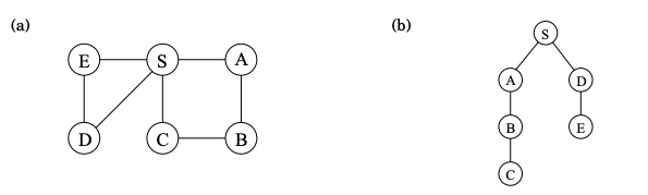
Breadth-first search (BFS)
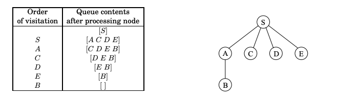
In BFS the lifting of the starting state , partitions the graph into layers: itself (vertex at distance 0), the vertices at distance 1 from it, the vertices at distance 2 from it etc.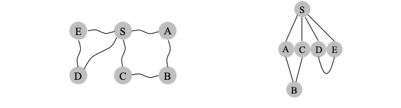
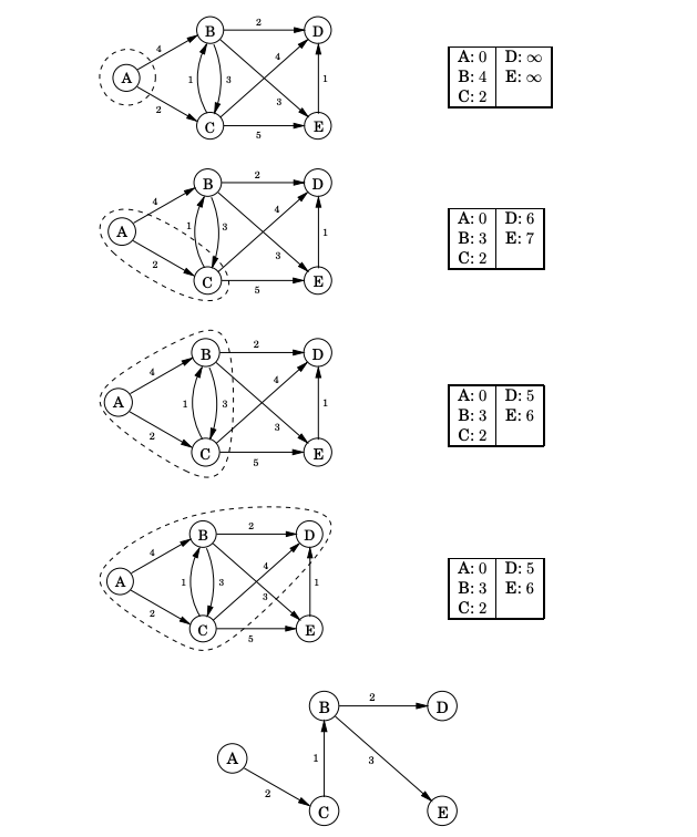
Dijkstra’s Algorithm
Breadth-first search finds shortest paths in any graph whose edges have unit length. Can we adapt it to a more general graph G = (V, E) whose edge lengths are positive integers? These lengths effectively represent the cost of traversing the edge. Here is a simple trick for converting G into something BFS can handle: break G’s long edges into unit-length pieces, by introducing “dummy” nodes as shown next.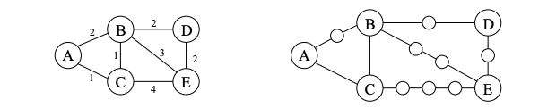

Found an error on this page? Report an issue.