If you are missing some algorithmic background, afraid not. There is a free and excellent book to help you with the background behind this chapter. Read Chapters 3 and 4 for the relevant background.
Given an initial state sIs_I (that can be represented in a graph by an initial node) and the goal state sGs_G (represented by a destination node) that is reached after potentially a finite number of actions (if a solution exist), we develop here a forward search algorithm whose pseudo-code is from Steven LaValle’s book - Chapter 2. The forward search uses two data structures, a priority queue (Q) and a list and proceeds as follows:
  1. Provided that the starting state is not the goal state, we add it to a priority queue called the frontier (also known as open list in the literature but we avoid using this term as it is implemented as a queue). The name frontier is synonymous to unexplored.
  2. We expand each state in our frontier, by applying the finite set of actions, generating a new list of states. We use a list that we call the explored set or closed list to remember each node (state) that we expanded.
  3. We then go over each newly generated state and before adding it to the frontier we check whether it has been explored before and in that case we discard it.

Forward-search approaches

The only significant difference between various search algorithms is the specific priority function that implements sQ.GetFirst()s \leftarrow Q.GetFirst() in other words the function that retrieves a state from the list of states held in the priority queue for expansion.
SearchQueue PolicyDetails
Depth-first search (DFS)LIFOSearch frontier is driven by aggressive exploration of the transition model. The algorithm makes deep incursions into the graph and retreats only when it run out of nodes to visit. It does not result in finding the shortest path to the goal.
Breath-first searchFIFOSearch frontier is expanding uniformly like the propagation of waves when you drop a stone in water. It therefore visit vertices in increasing order of their distance from the starting point.
DijkstraCost-to-Come or Past-Cost
A-starCost-to-Go or Future-Cost

Depth-first search (DFS)

In undirected graphs, depth-first search answers the question: What parts of the graph are reachable from a given vertex. It also finds explicit paths to these vertices, summarized in its search tree as shown below. depth-first Depth-first can’t find optimal (shortest) paths. Vertex C is reachable from S by traversing just one edge, while the DFS tree shows a path of length 3. On the right the DFS search tree is shown assuming alphabetical order in breaking up ties. Can you explain the DFS search tree? DFS can be run verbatim on directed graphs, taking care to traverse edges only in their prescribed directions.

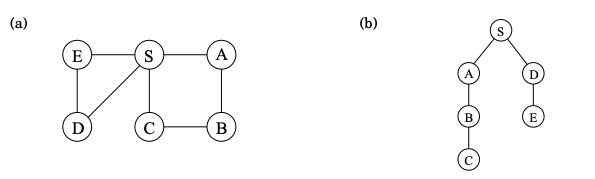
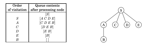
Breadth-first search (BFS)

In BFS the lifting of the starting state ss, partitions the graph into layers: ss itself (vertex at distance 0), the vertices at distance 1 from it, the vertices at distance 2 from it etc. breadth-first BFS expansion in terms of layers of vertices - each layer at increasing distance from the layer that follows. breadth-first-2 Queue contents during BFS and the BFS search tree assuming alphabetical order. Can you explain the BFS search tree? Is the BFS search tree a shortest-path tree?

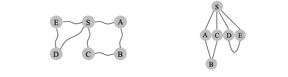
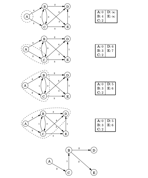
Dijkstra’s Algorithm

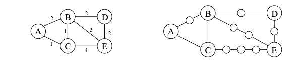
Breadth-first search finds shortest paths in any graph whose edges have unit length. Can we adapt it to a more general graph G = (V, E) whose edge lengths l(e)l(e) are positive integers? These lengths effectively represent the cost of traversing the edge. Here is a simple trick for converting G into something BFS can handle: break G’s long edges into unit-length pieces, by introducing “dummy” nodes as shown next. dijkstras-graph To construct the new graph GG' for any edge e=(s,s)e = (s, s^\prime) of EE, replace it by l(e)l(e) edges of length 1, by adding l(e)1l(e) − 1 dummy nodes between nodes ss and ss^\prime. With the shown transformation, we can now run BFS on GG' and the search tree will reveal the shortest path of each goal node from the starting point. The transformation allows us to solve the problem but it did result in an inefficient search where most of the nodes involved are searched but definitely will never be goal nodes. To look for more efficient ways to absorb the edge length l(e)l(e) we use the following as cost. search-cost-definitions Cost-to-come(ss) or PastCost(ss) vs. Cost-to-Go(ss) or FutureCost(ss). PastCost(ss) is the minimum cost from the start state sIs_I to state ss. FutureCost(ss) is the minimum cost from the state ss to the goal state sGs_G. The PastCost is used as the prioritization metric of the queue in Dijkstra’s algorithm. The addition of the PastCost with an estimate of the FutureCost, the heuristic h(s)h(s), i.e. G(s)=G(s) = PastCost(ss)+h(s)h(s), is used as the corresponding metric in the A* algorithm. What would be the ideal metric? The following example is instructive of the execution steps of the algorithm. dijkstras-example Example of Dijkstra’s algorithm execution steps and with sI=As_I=A The exact same pseudo-code is executed as before but the priority metric C(s)=C(s)+l(e)C(s^\prime)=C^*(s) + l(e) now accounts for costs as they are calculated causing the queue to be reordered accordingly. Here, C(s)C(s^\prime) represents the best cost-to-come that is known so far, but we do not write CC^* because it is not yet known whether ss^\prime was reached optimally. Due to this, some work is required in line: Resolve duplicate\texttt{Resolve duplicate} ss^\prime. If ss^\prime already exists in QQ, then it is possible that the newly discovered path to ss^\prime is more efficient. If so, then the cost-to-come value C(s)C(s^\prime) must be lowered for ss^\prime, and QQ must be reordered accordingly. When does C(s)C(s) finally become C(x)C^*(x) for some state ss? Once ss is removed from QQ using Q.GetFirst()Q.GetFirst(), the state becomes dead, and it is known that xx cannot be reached with a lower cost.
Connect these docs to Claude, VSCode, and more via MCP for real-time answers.