Introduction to RL

As we have seen in MDP, DP algorithms use full width backups. For example, in the tree representation of the value iteration algorithm shown below, every successor state and action is considered and evaluated using the known transition (environment dynamics) and reward functions. DP bootstraps the $v$ and $q$ function estimation from full-width backups. This can be feasible for moderate size problems but even a single backup cant be feasible when we have very large state spaces. So we definitely need to develop approaches that allow agents to

• optimally act in very large known MDPs or
• optimally act when we don’t know the MDP functions.

In this chapter we outline prediction and control methods that are basic building blocks behind both cases. We develop agents that can act in an initially unknown environment and learn via their interactions with it, gradually improving their policy. In the reinforcement learning problem setting, agents do not know essential elements of the MDP $\mathcal M = \langle \mathcal S, \mathcal P, \mathcal R, \mathcal A, \gamma \rangle$ that were assumed as given in fully observed MDP. This includes the transition function $P(s' \mid s, a)$ and the reward function $\mathcal R(s, a)$ that are essential as we have seen previously to estimate the value function and optimize the policy. The only way an agent can get information about these missing functions is through its experiences (states, actions, and rewards) in the environment—that is, the sequences of tuples ($S_t, A_t, R_{t+1}$). Provided that it can learn such functions, RL can be posed as an MDP and many concepts we have already covered in the MDP chapter still apply.

​

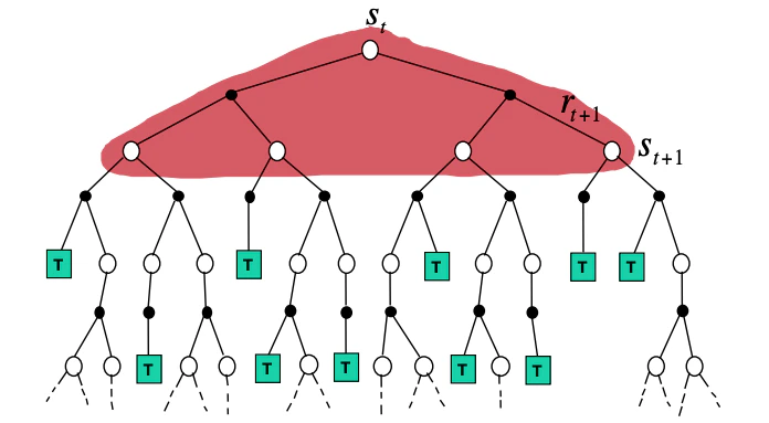
Future value calculation

Two natural questions arise

1. With what future states and actions we estimate the values,
2. How we control / schedule the updates to the values such that we can converge in an optimal policy at some point.

To answer the first question we look at the options we have with respect to the depth and width of the backup trees as shown in Different approaches to solving known and unknown MDPs. Several if not all RL algorithms are sampling the state-action space and use shallow to deep backups. To answer the second question we recall that in MDP the policy iteration consists of two simultaneous, interacting processes: one making the value function consistent with the current policy (policy evaluation), and the other making the policy greedy with respect to the current value function (policy improvement). In policy iteration these two processes alternate, each completing before the other begins. But this is not really necessary. In value iteration, for example, only a single sweep of policy evaluation is performed in between each policy improvement. In some cases a single state is updated in one process before returning to the other. As long as both processes continue to update all states, the ultimate result is typically the same: convergence to the optimal value function and an optimal policy. Policy evaluation and policy improvement can interact at any granularity — the result is still convergence to $v^*$ and $\pi^*$. We use the term generalized policy iteration (GPI) to refer to the general idea of letting policy-evaluation and policy-improvement processes interact, independent of the granularity and other details of the two processes. The evaluation and improvement processes in GPI can be viewed as both competing and cooperating. They compete in the sense that they pull in opposing directions: making the policy greedy with respect to the value function typically makes the value function incorrect for the changed policy, and making the value function consistent with the policy typically causes that policy no longer to be greedy. In the long run, however, these two processes interact to find a single joint solution — the optimal value function and an optimal policy. Generalized policy iteration diagram. Policy evaluation and policy improvement are shown as arrows: they compete but also cooperate to reach the joint optimum. We have seen this diagram in policy iteration where the arrows take the system all the way to achieving one of the two goals completely. In GPI one could also take smaller, incomplete steps toward each goal. In either case, the two processes together achieve the overall goal of optimality even though neither is attempting to achieve it directly. Almost all RL algorithms comply to this GPI principle.

​

From GPI to modern RL algorithms

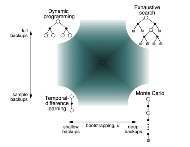
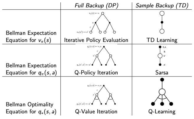
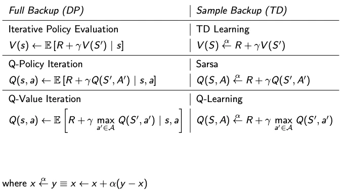
Three families of updates fit inside the GPI skeleton, and they differ along two orthogonal axes — width (full expectation vs. single sample) and depth (one step with bootstrapping vs. all the way to the end of the episode):

• DP uses full backups: it sweeps every successor $s'$ and weights by the known $P(s' \mid s, a)$. Requires a model.
• MC uses sample backups but waits for the episode to terminate and uses the actual return $G_t$. Model-free, unbiased, high variance.
• TD uses sample backups and bootstraps: one step of real experience plus the current estimate of $v$ or $Q$ at the next state. Model-free, biased, low variance.

Backup trees contrasting DP (full width, one step), MC (sample width, full depth), and TD (sample width, one step). Update equations: DP uses a weighted sum over all $s'$, MC uses the full return $G_t$, TD uses a bootstrapped one-step target $r + \gamma v(s')$.

​

Deep RL

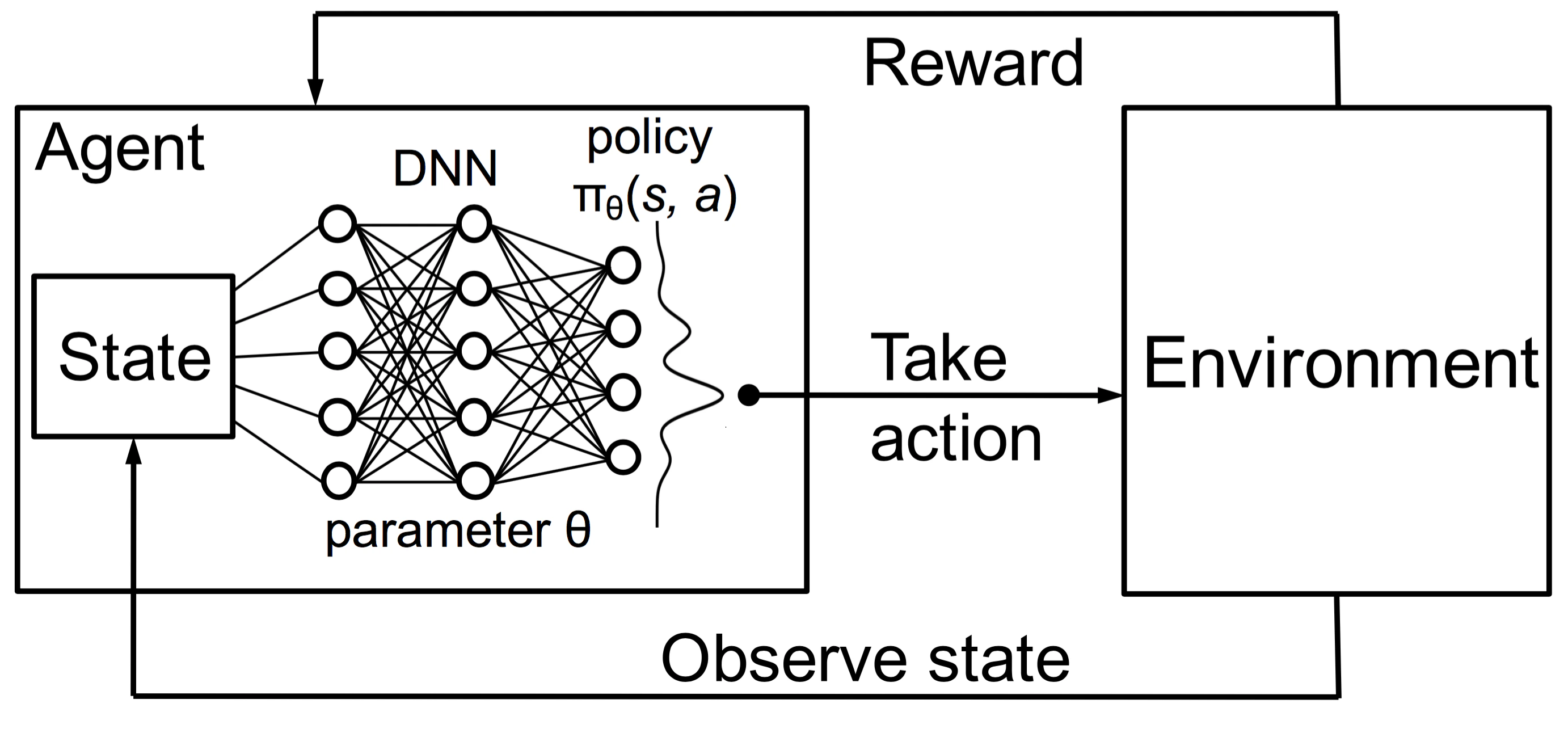
To scale to large problems, we also need to develop approaches that can learn such functions efficiently both in terms of computation and space (memory). We will use DNNs to provide, in the form of approximations, the needed efficiency boost. Deep Reinforcement Learning (DRL). DRL algorithms — taxonomy and evolution. In tabular DP, policy iteration and value iteration are two faces of the same algorithm — they both implement GPI and converge to the same $v^*$ and $\pi^*$. In modern RL each of them gave rise to its own algorithmic lineage: Value-iteration lineage — value-based RL. Q-learning (Watkins, 1989) is value iteration with the model replaced by samples and a max over actions in the bootstrap target. DQN (Mnih et al., 2015) is Q-learning with a neural-network function approximator and a replay buffer. From there follow double / dueling / distributional / rainbow DQN, R2D2, Agent57, and the value-prediction core of MuZero — all tracing back to the value-iteration update. Policy-iteration lineage — policy-gradient and actor-critic RL. Policy gradient methods (REINFORCE, A2C/A3C, TRPO, PPO, IMPALA) implement the “policy improvement” half via gradient ascent on the expected return rather than a greedy argmax. PPO is probably the most widely deployed modern RL algorithm today — it powers most of RLHF, robotics policies, and a lot of game-playing agents — and conceptually it is an approximate policy iteration: evaluate the current policy with rollouts, update with a clipped surrogate objective, repeat. Actor-critic methods like DDPG, TD3, and SAC literally implement GPI with neural-network policy and value heads — a critic trained with the value-iteration-style $\max_a$ bootstrap, and an actor improved by policy gradients. They inherit both lineages simultaneously.

​

Resources

The reader is encouraged to explore the following resources to get a better understanding of the DRL landscape.

1. Spinning Up in Deep RL. This is a must read for all computer scientists that are getting started in Deep RL.
2. Foundations of Deep RL. This is a practical book available for free via the O’Reilly .

Key references: (Schmidhuber, 2015; Li et al., 2015; Tamar et al., 2016; Tamar et al., 2016; Ma & Yu, 2016)

​

References

• Li, X., Li, L., Gao, J., He, X., Chen, J., et al. (2015). Recurrent Reinforcement Learning: A Hybrid Approach.
• Ma, S., Yu, J. (2016). Transition-based versus State-based Reward Functions for MDPs with Value-at-Risk.
• Schmidhuber, J. (2015). On Learning to Think: Algorithmic Information Theory for Novel Combinations of Reinforcement Learning Controllers and Recurrent Neural World Models.
• Tamar, A., Wu, Y., Thomas, G., Levine, S., Abbeel, P. (2016). Value Iteration Networks.
• Tamar, A., Wu, Y., Thomas, G., Levine, S., Abbeel, P. (2016). Value Iteration Networks.

---