Vision Transformers

A transformer takes a sequence of tokens. The transformer pages of the NLP chapter built one for text, where a tokenizer turns a sentence into a sequence of word pieces and an embedding table turns each piece into a vector. The vision transformer (ViT) of Dosovitskiy et al. applies the same encoder to images with one change at the input: the image is cut into square patches, and each patch becomes a token (Dosovitskiy et al., 2020). Everything after that step is the transformer you already know. This section builds a small ViT in PyTorch, piece by piece, and trains it on CIFAR-10. Along the way it answers the questions that the one-line summary hides. How does a patch become a vector? How does the model know where a patch was in the image, and what happens when the image size changes? Which token does the classifier read? Why did ViT need hundreds of millions of training images to beat a convolutional network, and what made it work on a data set of ordinary size? You need the attention mechanism from single-head and multi-head self-attention. The ViT encoder is the text encoder of the NLP chapter with the causal mask removed; cross-attention and position encoding explains the difference between an encoder and a decoder.

import math
import time

import numpy as np
import torch
import torch.nn.functional as F
from torch import nn

torch.manual_seed(0)
device = torch.device("cuda" if torch.cuda.is_available() else "cpu")
print(f"[INFO] device: {device}")

[INFO] device: cuda

Images as sequences of patches

32 \times 32

color image cut into patches of

P \times P = 4 \times 4

pixels gives an

8 \times 8

grid of patches,

N = 64

in total. Each patch holds

4 \cdot 4 \cdot 3 = 48

numbers. Flatten each patch into a vector

\mathbf{x}_i \in \mathbb{R}^{48}

and multiply it by a learned matrix

\mathbf{E} \in \mathbb{R}^{48 \times D}

to get a token of dimension

D

\mathbf{z}_i = \mathbf{x}_i \mathbf{E} + \mathbf{b}, \qquad i = 1, \dots, N.

The same

\mathbf{E}

is applied to every patch, just as the same embedding table is used for every word.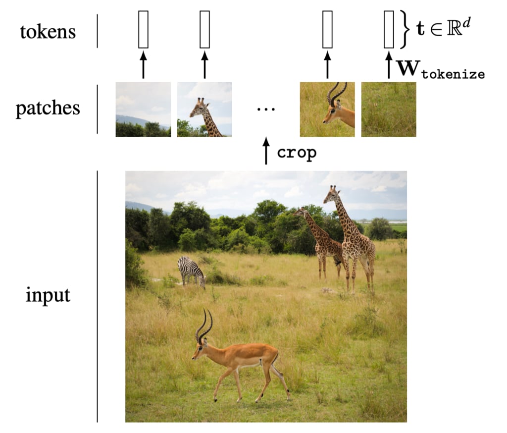

An image of a savanna is cropped into square patches, and each patch is mapped to a token vector t in R^d by a shared matrix W_tokenize.

Tokenizing an image: crop it into patches, then map each patch to a token with one shared linear map. Figure from Torralba, Isola and Freeman (Foundations of Computer Vision, n.d.). A linear map applied to non-overlapping

P \times P

windows is a convolution with kernel size

P

and stride

P

, so implementations write the patch embedding as nn.Conv2d. The cell below checks that the two give the same tokens when the convolution kernel is the matrix

\mathbf{E}

reshaped.

P, C, D = 4, 3, 192
conv = nn.Conv2d(C, D, kernel_size=P, stride=P)

x = torch.randn(2, C, 32, 32)  # a batch of two images

# Patch embedding with the convolution: (B, D, 8, 8) -> (B, 64, D)
tokens_conv = conv(x).flatten(2).transpose(1, 2)

# Patch embedding by hand: cut the patches, flatten them, multiply by E
patches = x.unfold(2, P, P).unfold(3, P, P)                # (B, C, 8, 8, P, P)
patches = patches.permute(0, 2, 3, 1, 4, 5).reshape(2, 64, C * P * P)
E = conv.weight.reshape(D, C * P * P).T                     # (48, D)
tokens_linear = patches @ E + conv.bias

print("tokens:", tuple(tokens_conv.shape))
print("largest difference:", (tokens_conv - tokens_linear).abs().max().item())

tokens: (2, 64, 192)
largest difference: 5.960464477539062e-07

The two agree to rounding error. The convolution is only a faster way to compute the same linear map.

The [CLS] token and position embeddings

Two things are still missing before the tokens can enter the encoder. The first is a place to read the answer from. ViT follows BERT and adds one extra learned vector, the class token [CLS], at the start of the sequence. It corresponds to no patch. Through attention it collects information from all the patch tokens, and after the last layer a linear classifier reads only the [CLS] output. The alternative is to average the outputs of all patch tokens (mean pooling) and classify the average. Both work, and the experiments below compare them. The second is position. Self-attention is permutation equivariant: shuffle the input tokens and the outputs are shuffled the same way, with no other change. Without extra information the encoder could not tell a patch in the top-left corner from the same patch in the bottom-right. ViT adds a learned vector

\mathbf{p}_i

to each token, one per position:

\mathbf{z}^{(0)} = [\mathbf{z}_{\text{cls}};\ \mathbf{x}_1\mathbf{E} + \mathbf{b};\ \dots;\ \mathbf{x}_N\mathbf{E} + \mathbf{b}] + [\mathbf{p}_0; \mathbf{p}_1; \dots; \mathbf{p}_N].

The positions are numbered

1, \dots, N

along the rows of the grid, so the model is not told that position 9 is directly below position 1. It has to learn the 2D layout from data. Dosovitskiy et al. tried position embeddings that encode the row and column explicitly and found no clear gain over this 1D version. After training, the learned embeddings of neighboring patches are similar, which the plot near the end of this section shows.

class PatchEmbedding(nn.Module):
    # Image (B, C, H, W) -> patch tokens (B, N, D)
    def __init__(self, in_channels=3, patch_size=4, emb_size=192):
        super().__init__()
        self.proj = nn.Conv2d(in_channels, emb_size, kernel_size=patch_size, stride=patch_size)

    def forward(self, x):
        return self.proj(x).flatten(2).transpose(1, 2)

The encoder block

Each encoder block is the one from the NLP chapter: layer normalization, multi-head self-attention and a residual connection, then layer normalization, a two-layer MLP applied to each token separately and a second residual connection. ViT puts the normalization before each sublayer (pre-norm), which trains more stably than the post-norm layout of the original transformer.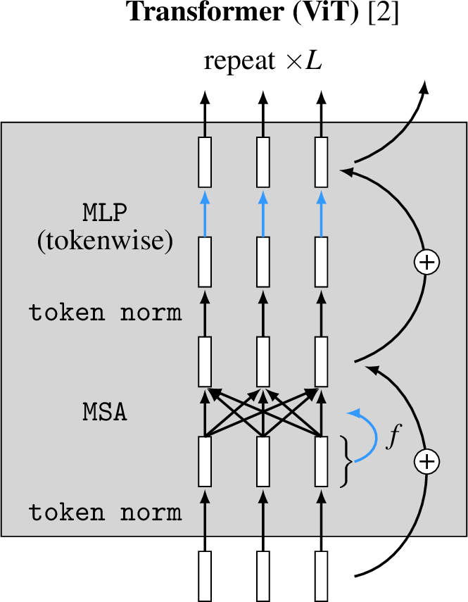

One ViT block: token norm, multi-head self-attention mixing all tokens, a residual connection, token norm, a tokenwise MLP and a second residual connection, repeated L times.

One ViT encoder block, repeated $L$ times. Figure from Torralba, Isola and Freeman (Foundations of Computer Vision, n.d.). There is no causal mask. In a decoder that generates text, token

i

may only attend to tokens

1, \dots, i

, because the later tokens do not exist yet when token

i

is produced. An image is available all at once, so every patch attends to every other patch in both directions. PyTorch’s nn.MultiheadAttention expects its input as (sequence, batch, features) unless it is created with batch_first=True. The tokens here are (batch, sequence, features). Without the flag, the layer reads the batch axis as the sequence axis, and each token attends to the tokens at the same position in the other images of the batch instead of the other patches of its own image. The model still runs and still trains, but it cannot learn anything useful, and its accuracy stays at chance. An earlier version of this section had exactly this bug.

class EncoderBlock(nn.Module):
    def __init__(self, emb_size, num_heads, mlp_ratio=4, dropout=0.0):
        super().__init__()
        self.norm1 = nn.LayerNorm(emb_size)
        self.attn = nn.MultiheadAttention(emb_size, num_heads, dropout=dropout, batch_first=True)
        self.norm2 = nn.LayerNorm(emb_size)
        self.mlp = nn.Sequential(
            nn.Linear(emb_size, mlp_ratio * emb_size),
            nn.GELU(),
            nn.Linear(mlp_ratio * emb_size, emb_size),
            nn.Dropout(dropout),
        )
        self.keep_attention = False  # set to True to store the attention weights
        self.attention = None

    def forward(self, x):
        h = self.norm1(x)
        out, weights = self.attn(h, h, h, need_weights=self.keep_attention,
                                 average_attn_weights=True)
        if self.keep_attention:
            self.attention = weights  # (B, N+1, N+1), averaged over the heads
        x = x + out
        x = x + self.mlp(self.norm2(x))
        return x

The full model

The model chains the pieces: patch embedding, [CLS] token, position embeddings,

L

encoder blocks, a final layer norm and a linear head. The pool argument chooses whether the head reads the [CLS] output or the mean of the patch outputs. The configuration is a small one for

32 \times 32

images: patches of

4 \times 4

pixels (64 tokens plus [CLS]),

D = 192

, 3 heads and 6 blocks, about 2.7 million parameters. ViT-Base, the model of the paper, uses

16 \times 16

patches on

224 \times 224

images (196 tokens),

D = 768

, 12 heads and 12 blocks, 86 million parameters. On a

32 \times 32

image a

16 \times 16

patch would leave only four tokens, which is why the patch size shrinks with the image.

class ViT(nn.Module):
    def __init__(self, img_size=32, patch_size=4, in_channels=3, num_classes=10,
                 emb_size=192, depth=6, num_heads=3, mlp_ratio=4, dropout=0.0, pool="cls"):
        super().__init__()
        self.grid = img_size // patch_size
        self.pool = pool
        self.patch_embed = PatchEmbedding(in_channels, patch_size, emb_size)
        self.cls_token = nn.Parameter(torch.zeros(1, 1, emb_size))
        self.pos_embed = nn.Parameter(torch.randn(1, self.grid * self.grid + 1, emb_size) * 0.02)
        self.blocks = nn.ModuleList(
            [EncoderBlock(emb_size, num_heads, mlp_ratio, dropout) for _ in range(depth)]
        )
        self.norm = nn.LayerNorm(emb_size)
        self.head = nn.Linear(emb_size, num_classes)

    def forward(self, x, pos_embed=None):
        x = self.patch_embed(x)                                   # (B, N, D)
        cls = self.cls_token.expand(x.shape[0], -1, -1)
        x = torch.cat([cls, x], dim=1)                            # (B, N+1, D)
        x = x + (self.pos_embed if pos_embed is None else pos_embed)
        for block in self.blocks:
            x = block(x)
        x = self.norm(x)
        features = x[:, 0] if self.pool == "cls" else x[:, 1:].mean(dim=1)
        return self.head(features)


model = ViT()
print(f"[INFO] parameters: {sum(p.numel() for p in model.parameters()):,}")
print("[INFO] logits:", tuple(model(torch.randn(2, 3, 32, 32)).shape))

[INFO] parameters: 2,693,578
[INFO] logits: (2, 10)

Inductive bias and data

A convolutional network builds two assumptions about images into its architecture. A convolution looks at a small neighborhood, so the network starts from local features (locality). The same kernel slides over the whole image, so a pattern is detected the same way wherever it appears (translation equivariance). These assumptions are the network’s inductive bias. They are right for most images, and they let a CNN learn from a modest data set. A ViT has almost none of this. Only the patch embedding is local, and every attention layer can connect any patch to any other from the first block on. Which patches matter for which, and the fact that nearby patches tend to belong together, must be learned from the data. Dosovitskiy et al. found that ViT trained on ImageNet-1k (1.3 million images) was a few points less accurate than a ResNet of similar size. Pretrained on ImageNet-21k (14 million) the two were close, and pretrained on JFT-300M (300 million) ViT was more accurate. With enough data, learning the structure works better than assuming it. Touvron et al. then showed that a ViT can reach ResNet accuracy when trained on ImageNet-1k alone, if the training adds strong data augmentation and regularization (DeiT, arXiv:2012.12877). Augmentation makes up for missing data: each random crop or flip is a new image with the same label, and it teaches the model that the label does not depend on the exact position of the object, which is the assumption that a CNN gets from its architecture. CIFAR-10 has 50,000 training images, far fewer than ImageNet, so the effect should be visible here. The experiment below trains the same ViT three times: without augmentation, with random crops and horizontal flips, and with augmentation and mean pooling instead of [CLS].

Training on CIFAR-10

The 50,000 training images are split into 45,000 for training and 5,000 for validation. The test set is used once, at the end. Each run trains for 30 epochs with AdamW, a learning rate that rises for two epochs and then decays along a cosine, and bfloat16 arithmetic on the GPU.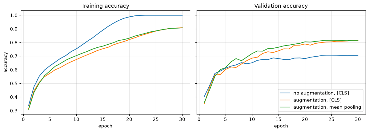

from torch.utils.data import DataLoader, Subset
from torchvision import datasets, transforms

MEAN, STD = (0.4914, 0.4822, 0.4465), (0.2470, 0.2435, 0.2616)
plain = transforms.Compose([transforms.ToTensor(), transforms.Normalize(MEAN, STD)])
augmented = transforms.Compose([
    transforms.RandomCrop(32, padding=4),
    transforms.RandomHorizontalFlip(),
    transforms.ToTensor(),
    transforms.Normalize(MEAN, STD),
])

train_plain = datasets.CIFAR10("data", train=True, download=True, transform=plain)
train_aug = datasets.CIFAR10("data", train=True, download=True, transform=augmented)
test_set = datasets.CIFAR10("data", train=False, download=True, transform=plain)

# The same 45,000 / 5,000 split for every run
perm = torch.randperm(len(train_plain), generator=torch.Generator().manual_seed(0))
train_idx, val_idx = perm[:45_000].tolist(), perm[45_000:].tolist()
val_set = Subset(train_plain, val_idx)  # validation images are never augmented
CLASSES = train_plain.classes
print(f"[INFO] train {len(train_idx):,}  validation {len(val_idx):,}  test {len(test_set):,}")

[INFO] train 45,000  validation 5,000  test 10,000

EPOCHS = 30
BATCH_SIZE = 256


def loader(dataset, shuffle):
    return DataLoader(dataset, batch_size=BATCH_SIZE, shuffle=shuffle, num_workers=4,
                      pin_memory=True, persistent_workers=True)


@torch.no_grad()
def evaluate(model, data, pos_embed=None, resize=None):
    model.eval()
    correct = total = 0
    for images, labels in data:
        images, labels = images.to(device), labels.to(device)
        if resize is not None:
            images = F.interpolate(images, size=resize, mode="bilinear", align_corners=False)
        with torch.autocast(device.type, dtype=torch.bfloat16):
            logits = model(images, pos_embed=pos_embed)
        correct += (logits.argmax(1) == labels).sum().item()
        total += labels.numel()
    return correct / total


def train_run(name, train_data, pool="cls", epochs=EPOCHS):
    torch.manual_seed(0)
    model = ViT(pool=pool).to(device)
    opt = torch.optim.AdamW(model.parameters(), lr=1e-3, weight_decay=0.05)
    train_loader = loader(Subset(train_data, train_idx), shuffle=True)
    val_loader = loader(val_set, shuffle=False)
    steps, warmup = epochs * len(train_loader), 2 * len(train_loader)
    sched = torch.optim.lr_scheduler.LambdaLR(
        opt, lambda s: (s + 1) / warmup if s < warmup
        else 0.5 * (1 + math.cos(math.pi * (s - warmup) / (steps - warmup))))
    history = {"train_acc": [], "val_acc": []}
    start = time.time()
    for epoch in range(epochs):
        model.train()
        correct = total = 0
        for images, labels in train_loader:
            images, labels = images.to(device), labels.to(device)
            with torch.autocast(device.type, dtype=torch.bfloat16):
                logits = model(images)
                loss = F.cross_entropy(logits, labels)
            opt.zero_grad(set_to_none=True)
            loss.backward()
            opt.step()
            sched.step()
            correct += (logits.argmax(1) == labels).sum().item()
            total += labels.numel()
        history["train_acc"].append(correct / total)
        history["val_acc"].append(evaluate(model, val_loader))
    print(f"{name:<28} train {history['train_acc'][-1]:.3f}  validation {history['val_acc'][-1]:.3f}"
          f"  ({time.time() - start:.0f} s)")
    return model, history

runs = {}
runs["no augmentation, [CLS]"] = train_run("no augmentation, [CLS]", train_plain, pool="cls")
runs["augmentation, [CLS]"] = train_run("augmentation, [CLS]", train_aug, pool="cls")
runs["augmentation, mean pooling"] = train_run("augmentation, mean pooling", train_aug, pool="mean")

no augmentation, [CLS]       train 1.000  validation 0.703  (86 s)

augmentation, [CLS]          train 0.908  validation 0.814  (88 s)

augmentation, mean pooling   train 0.907  validation 0.816  (88 s)

Without augmentation the model reaches 100% training accuracy by epoch 23, and its validation accuracy stops at 70.3%: it has memorized the 45,000 training images. Random crops and flips keep the training accuracy at 91% and raise the validation accuracy to 81.4%, eleven points more with the same model and the same number of steps. Mean pooling gives 81.6%, which is the same within the noise of a single run. On this problem the readout matters far less than the data.

best_name = max(runs, key=lambda n: runs[n][1]["val_acc"][-1])
best_model = runs[best_name][0]
test_loader = loader(test_set, shuffle=False)
print(f"[INFO] {best_name}: test accuracy {evaluate(best_model, test_loader):.3f}")

[INFO] augmentation, mean pooling: test accuracy 0.826

The run with the best validation accuracy reaches 82.6% on the test set, close to its validation accuracy, so the validation split was a fair guide to the choice.

What the position embeddings learned

Each position embedding is a vector of 192 numbers, and nothing in their initialization says that position 1 is next to position 2 or position 9. The plot shows, for each of the 64 patch positions, the cosine similarity of its embedding with the embeddings of all 64 positions, laid out on the

8 \times 8

grid. Each small square belongs to one position, and it is brightest at that position itself.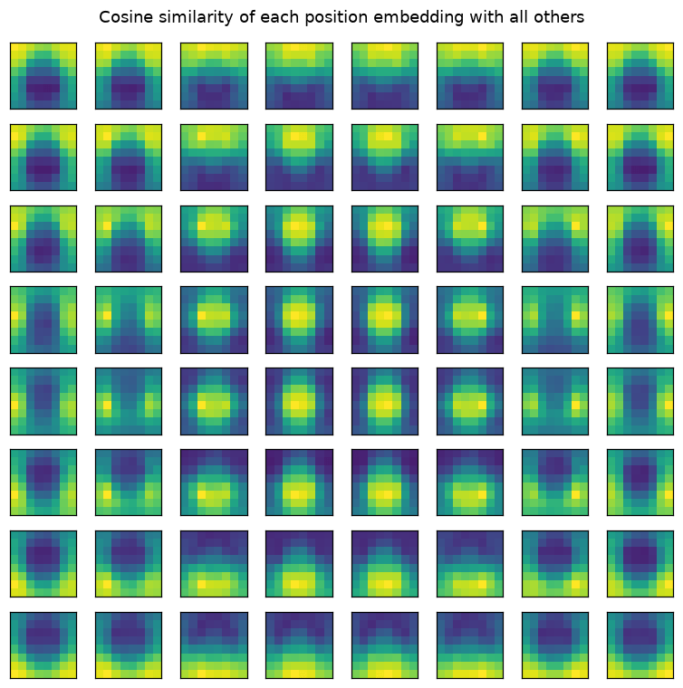

Each small square is brightest at its own position and fades with distance, along the rows and along the columns. The model has learned the 2D layout of the grid from the data, although the positions were numbered in one dimension. The squares are also symmetric from left to right: a position in the first column is similar to the mirrored position in the last column. That comes from the horizontal flips of the augmentation. A patch at the left edge of a training image sits at the right edge of its flipped copy, so the model gains nothing from telling the two apart.

Changing the image resolution

The position embeddings tie the model to one grid size. A

48 \times 48

image cut into

4 \times 4

patches gives a

12 \times 12

grid, 144 tokens, and the model has embeddings for only 64. The standard fix, used when a ViT pretrained at one resolution is fine-tuned at a higher one, is to treat the 64 patch embeddings as an

8 \times 8

image with 192 channels and resize it to

12 \times 12

with bicubic interpolation. The [CLS] embedding is kept as it is. The cell evaluates the best model on validation images upsampled to

48 \times 48

, once with interpolated position embeddings and, for comparison, at the original

32 \times 32

def resize_pos_embed(pos_embed, old_grid, new_grid):
    # Interpolate the patch position embeddings from old_grid x old_grid to new_grid x new_grid
    cls, grid = pos_embed[:, :1], pos_embed[:, 1:]
    D = grid.shape[-1]
    grid = grid.reshape(1, old_grid, old_grid, D).permute(0, 3, 1, 2)      # (1, D, 8, 8)
    grid = F.interpolate(grid, size=(new_grid, new_grid), mode="bicubic", align_corners=False)
    grid = grid.permute(0, 2, 3, 1).reshape(1, new_grid * new_grid, D)
    return torch.cat([cls, grid], dim=1)


val_loader = loader(val_set, shuffle=False)
pos48 = resize_pos_embed(best_model.pos_embed, 8, 12)
print(f"[INFO] 32 x 32, 64 patch tokens:  validation accuracy {evaluate(best_model, val_loader):.3f}")
print(f"[INFO] 48 x 48, 144 patch tokens: validation accuracy "
      f"{evaluate(best_model, val_loader, pos_embed=pos48, resize=48):.3f}")

[INFO] 32 x 32, 64 patch tokens:  validation accuracy 0.816
[INFO] 48 x 48, 144 patch tokens: validation accuracy 0.602

With interpolated position embeddings the model still runs on

48 \times 48

inputs and reaches 60.2%, far above the 10% of chance but well below the 81.6% at the training resolution. Each

4 \times 4

patch now covers a smaller part of the object than it did during training, so the patch embedding sees details at a different scale. This is why a ViT that moves to a higher resolution is fine-tuned for a few epochs at the new size, starting from the interpolated embeddings.

Attention maps

The attention weights of the [CLS] token in the last block show which patches the classifier’s input was built from. For each image below, the weights of the [CLS] query over the 64 patches, averaged over the heads, are reshaped to the

8 \times 8

grid and drawn over the image. These maps come from a single layer of a small model, so they are a rough picture. Methods such as attention rollout combine the maps of all layers.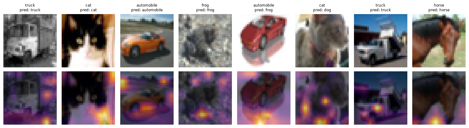

cls_model = runs["augmentation, [CLS]"][0]
last = cls_model.blocks[-1]
last.keep_attention = True

images, labels = next(iter(loader(val_set, shuffle=False)))
images = images[:8].to(device)
with torch.no_grad():
    predictions = cls_model(images).argmax(1).cpu()
cls_attention = last.attention[:, 0, 1:].reshape(-1, 8, 8).float().cpu()  # [CLS] row, patch columns
last.keep_attention = False

The maps do not outline the objects. In most images the [CLS] token attends to a few small spots, often at the border or in the background, such as the bottom edge of the truck and frog images. Six of the eight images are classified correctly; the red car on a white background is called a frog, and the cat with a collar a dog. By the last layer, every patch token already mixes information from the whole image through five earlier layers of attention, so the spot that the [CLS] token reads need not be where the object is. The attention map of a single layer is therefore a weak explanation of what the model used.

Exercises

Train the model for 30 epochs with patches of $8 \times 8$ pixels (16 tokens) and $2 \times 2$ pixels (256 tokens). Report the validation accuracy and the training time per epoch, and explain both with the cost of attention, which grows with the square of the number of tokens.
Remove the position embeddings (set them to zero and freeze them). How much accuracy does the model lose? Then shuffle the patch order of every validation image with one fixed permutation and evaluate the model with and without position embeddings. Explain the result with permutation equivariance.
Replace the 1D position embeddings with 2D ones: one learned vector per row and one per column, each of dimension $D/2$ , concatenated. Compare the accuracy and the similarity plot with the 1D version.
Add a stronger augmentation, such as transforms.RandAugment(), and train for 60 epochs. Does the gap to the run without augmentation keep growing with longer training?
Train a small CNN with about the same number of parameters on the same split and with the same augmentation. Which is more accurate after 30 epochs, and how does the answer relate to inductive bias?

Key references

Dosovitskiy et al. introduced the vision transformer and measured how its accuracy depends on the size of the pretraining data (Dosovitskiy et al., 2020). Chapter 26 of Torralba, Isola and Freeman explains tokens and attention for images (Foundations of Computer Vision, n.d.).

PyTorch reference

PyTorch class	Description
`nn.Conv2d`	Applies a 2D convolution over an input signal composed of several input planes.
`nn.MultiheadAttention`	Allows the model to jointly attend to information from different representation subspaces.
`nn.LayerNorm`	Applies Layer Normalization over a mini-batch of inputs.
`nn.Linear`	Applies an affine linear transformation to the incoming data: $y = xA^T + b$ .
`nn.GELU`	Applies the Gaussian Error Linear Units function.
`nn.Dropout`	During training, randomly zeroes some of the elements of the input tensor with probability p.

References

Dosovitskiy, A., Beyer, L., Kolesnikov, A., Weissenborn, D., Zhai, X., et al. (2020). An Image is Worth 16x16 Words: Transformers for Image Recognition at Scale. arXiv [cs.CV].
(n.d.). Foundations of Computer Vision.

Found an error on this page? Report an issue.

Vision and Language