3D Motion and Its 2D Projection

This section was written by Kaushik Kachireddy (pull request #73), with help from an AI coding agent (Claude Code) on the code. It reproduces the ideas of Chapter 47 of Foundations of Computer Vision by Antonio Torralba, Phillip Isola, and William T. Freeman. When a 3D point moves, or the camera moves, how does its image on the camera plane move? This section answers that question with one long derivation: the motion field equation (47.8). Once you have it, every interesting motion phenomenon falls out as a special case: vanishing points, parallax, the focus of expansion, time-to-contact, and the way a zoom looks different from a dolly. Each figure here is a diagram or a sketch of a vector field, drawn by encoding the underlying math in PyTorch. There are no photographs.

import torch
import matplotlib.pyplot as plt
from matplotlib.patches import Polygon, Rectangle, Circle, FancyArrowPatch, PathPatch
from matplotlib.path import Path
from mpl_toolkits.mplot3d import Axes3D  # noqa: F401, registers 3d projection

torch.set_default_dtype(torch.float32)
_ = torch.manual_seed(0)

Perspective projection of a moving point

A 3D point

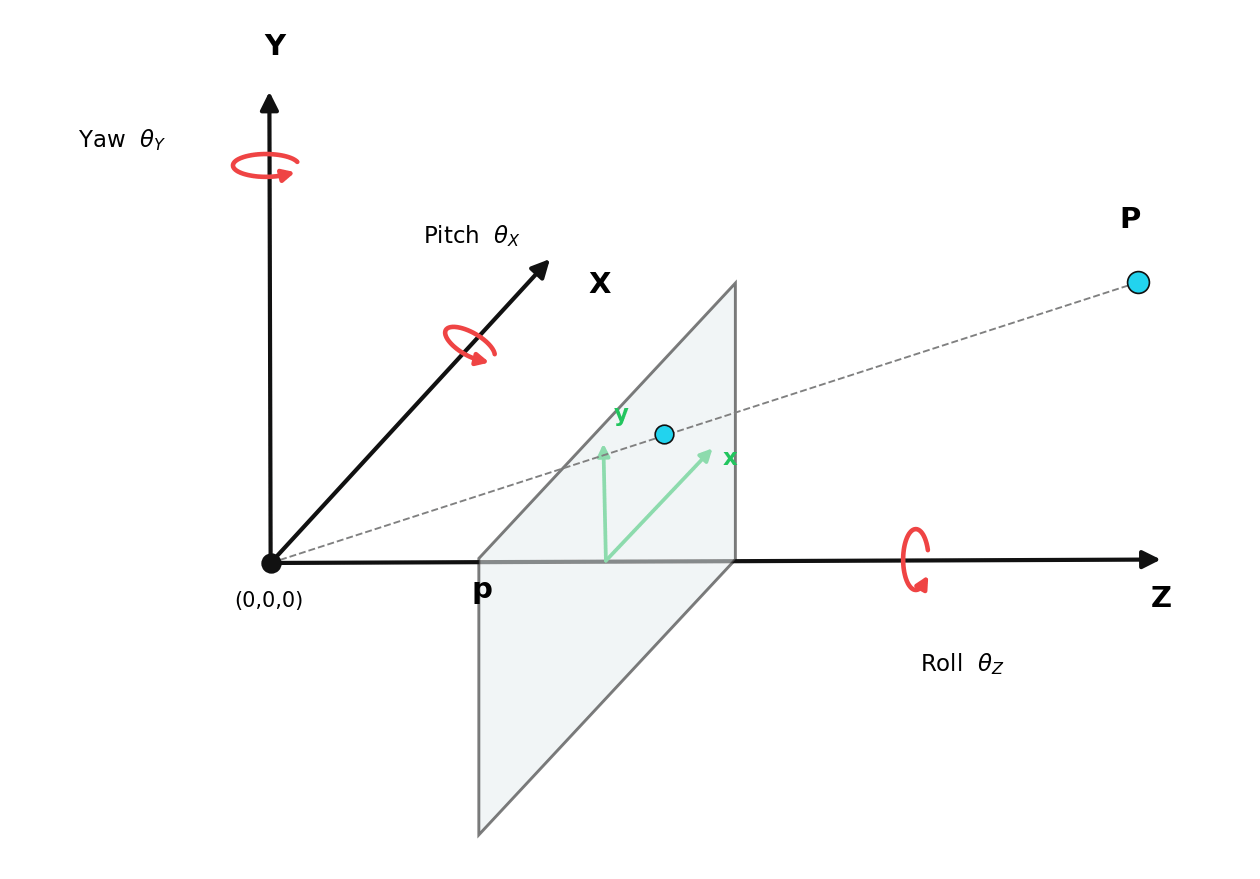
\mathbf{P} = (X, Y, Z)

projects to image coordinates

\mathbf{p} = (x, y)

through the pinhole camera with focal length

f

(equation 47.9):

x = f\,\frac{X}{Z}, \qquad y = f\,\frac{Y}{Z}.

When

\mathbf{P}

moves with velocity

\dot{\mathbf{P}} = (\dot X, \dot Y, \dot Z)

, the image point moves too. Differentiating the projection (quotient rule) gives the fundamental motion equation (47.1):

\begin{bmatrix}\dot x\\\dot y\end{bmatrix} = \frac{1}{Z}\begin{bmatrix} f & 0 & -x \\ 0 & f & -y \end{bmatrix}\begin{bmatrix}\dot X\\\dot Y\\\dot Z\end{bmatrix}.

The

1/Z

factor is the entire reason vision can recover depth from motion, because closer points produce larger image-plane velocities than farther points moving the same way.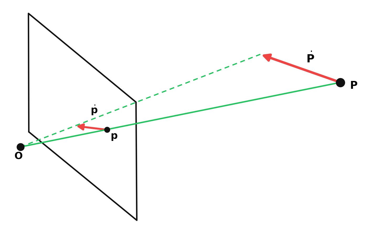

def project(P, f=1.0):
    """Pinhole projection (Eq. 47.9). P shape: (..., 3) → (..., 2)."""
    X, Y, Z = P[..., 0], P[..., 1], P[..., 2]
    return torch.stack([f * X / Z, f * Y / Z], dim=-1)


def project_velocity(P, P_dot, f=1.0):
    """Image-plane velocity from 3D point + 3D velocity (Eq. 47.1)."""
    X, Y, Z = P[..., 0], P[..., 1], P[..., 2]
    Xd, Yd, Zd = P_dot[..., 0], P_dot[..., 1], P_dot[..., 2]
    x = f * X / Z
    y = f * Y / Z
    xd = (f * Xd - x * Zd) / Z
    yd = (f * Yd - y * Zd) / Z
    return torch.stack([xd, yd], dim=-1)

Two easy cases of equation 47.1

Equation 47.1 has three terms. Killing one at a time isolates the two simplest motion regimes: Motion parallel to the image plane (

\dot Z = 0

, equation 47.2):

\begin{bmatrix}\dot x\\\dot y\end{bmatrix} = \frac{f}{Z}\begin{bmatrix}\dot X\\\dot Y\end{bmatrix}.

The magnitude is inversely proportional to depth: pure parallax. Motion along the optical axis (

\dot X = \dot Y = 0

, equation 47.3):

\begin{bmatrix}\dot x\\\dot y\end{bmatrix} = -\frac{\dot Z}{Z}\begin{bmatrix}x\\y\end{bmatrix}.

Motion is radial, scaled by the ratio

\dot Z / Z

(the time-to-contact). Figure 47.2 sketches both.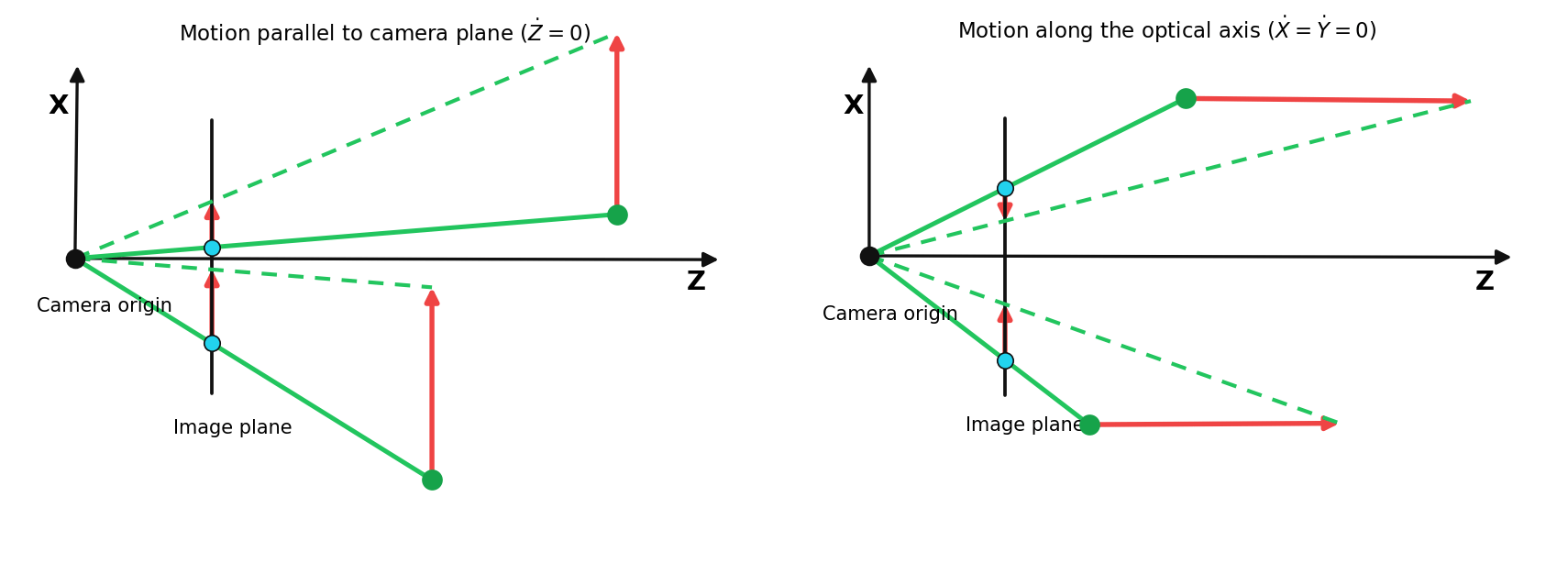

The vanishing point

Let a point move with constant world velocity

\mathbf{V} = (V_X, V_Y, V_Z)

from initial position

\mathbf{P}_0

. Its position is

\mathbf{P}(t) = \mathbf{P}_0 + t\mathbf{V}

, and its image is

\mathbf{p}(t) = \frac{f}{P_{0,Z} + tV_Z}\begin{bmatrix}P_{0,X} + tV_X \\ P_{0,Y} + tV_Y\end{bmatrix}.

t \to \infty

the initial-position terms drop out and you land at the vanishing point (equation 47.4):

x_{\infty} = f\,\frac{V_X}{V_Z},\qquad y_{\infty} = f\,\frac{V_Y}{V_Z}.

The vanishing point depends only on the direction of motion, never on where the point started. Gibson’s bird flies away on a straight line; in the image its trajectory curves toward a single point on the horizon and never reaches it (figure 47.3).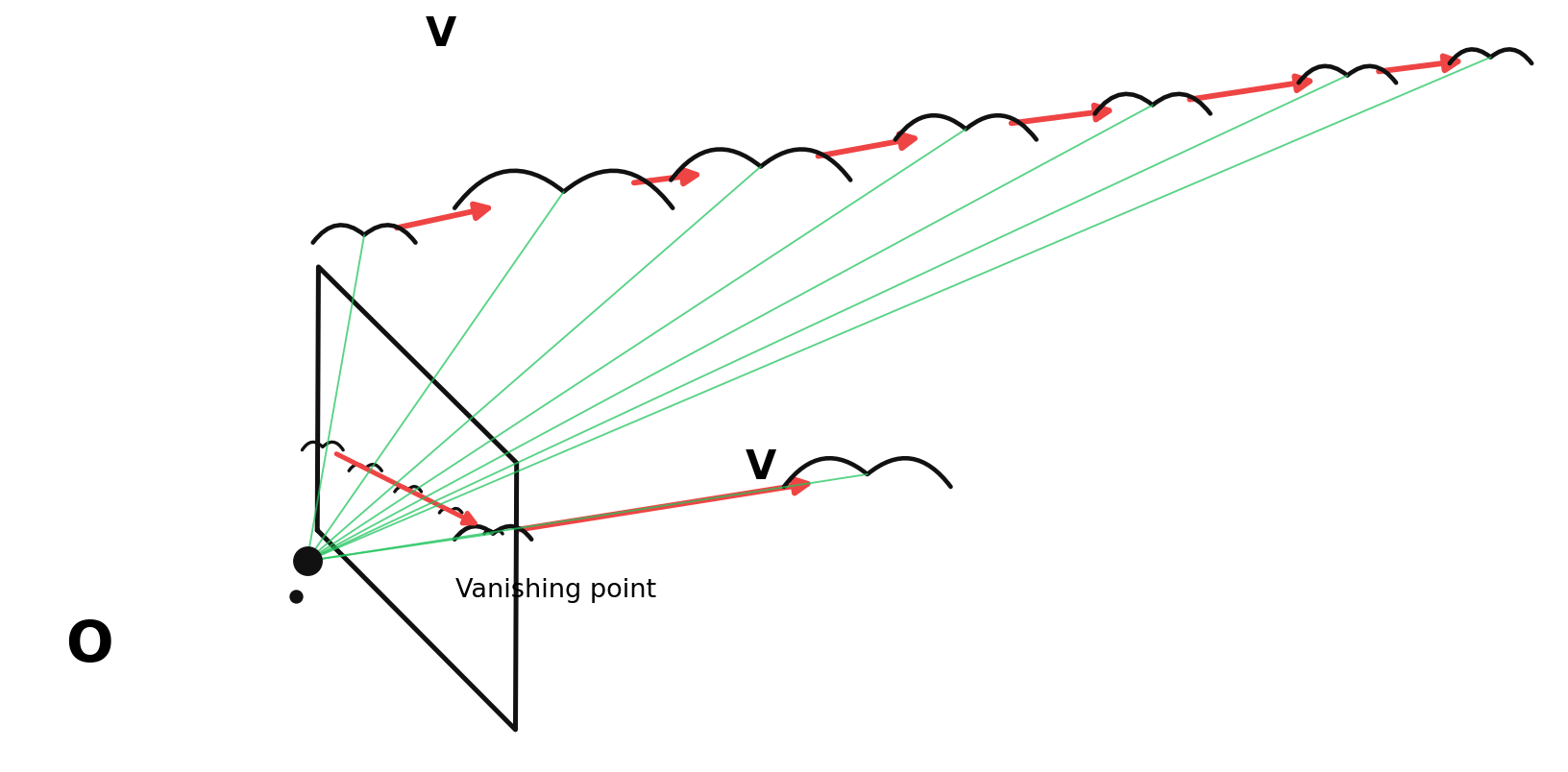

The motion field under camera translation

When the camera translates with velocity

\mathbf{V}

through a static world, each scene point moves with

-\mathbf{V}

in the camera frame. Substituting

\dot{\mathbf{P}} = -\mathbf{V}

into equation 47.1 gives the camera-translation motion field (equation 47.5):

\begin{bmatrix}\dot x\\\dot y\end{bmatrix} = \frac{1}{Z}\begin{bmatrix}-f & 0 & x\\0 & -f & y\end{bmatrix}\begin{bmatrix}V_X\\V_Y\\V_Z\end{bmatrix}.

The full motion field including rotation is given by equation 47.8, which the next cell encodes once and every later figure reuses.

def motion_field(x, y, Z, V, W, f=1.0):
    """Full image-plane motion field (Eq. 47.8).

    Args:
        x, y: image-plane coordinates, same shape.
        Z:    scene depth at each (x, y), broadcastable to x.
        V:    (3,) camera translational velocity (V_X, V_Y, V_Z).
        W:    (3,) camera angular velocity (W_X, W_Y, W_Z).
        f:    focal length.
    Returns:
        (xdot, ydot): same shape as x.
    """
    Vx, Vy, Vz = V
    Wx, Wy, Wz = W
    trans_x = (-f * Vx + x * Vz) / Z
    trans_y = (-f * Vy + y * Vz) / Z
    rot_x = (x * y * Wx - (f * f + x * x) * Wy + f * y * Wz) / f
    rot_y = ((f * f + y * y) * Wx - x * y * Wy - f * x * Wz) / f
    return trans_x + rot_x, trans_y + rot_y


def image_grid(nx=15, ny=11, half_x=1.0, half_y=0.7):
    """A regular grid of image-plane sample points for quiver plots."""
    xs = torch.linspace(-half_x, half_x, nx)
    ys = torch.linspace(-half_y, half_y, ny)
    gx, gy = torch.meshgrid(xs, ys, indexing="xy")
    return gx, gy

Lateral camera motion

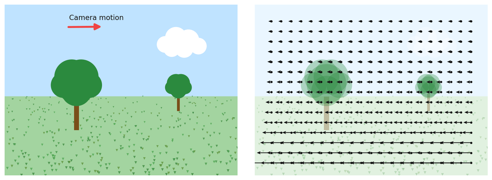
Driving past a roadside scene:

V_X \ne 0

V_Y = V_Z = 0

. The motion field collapses to

\dot x = -\frac{f V_X}{Z}, \qquad \dot y = 0.

Image-plane speed is inversely proportional to scene depth: close objects whip past while distant clouds barely move (figure 47.5).

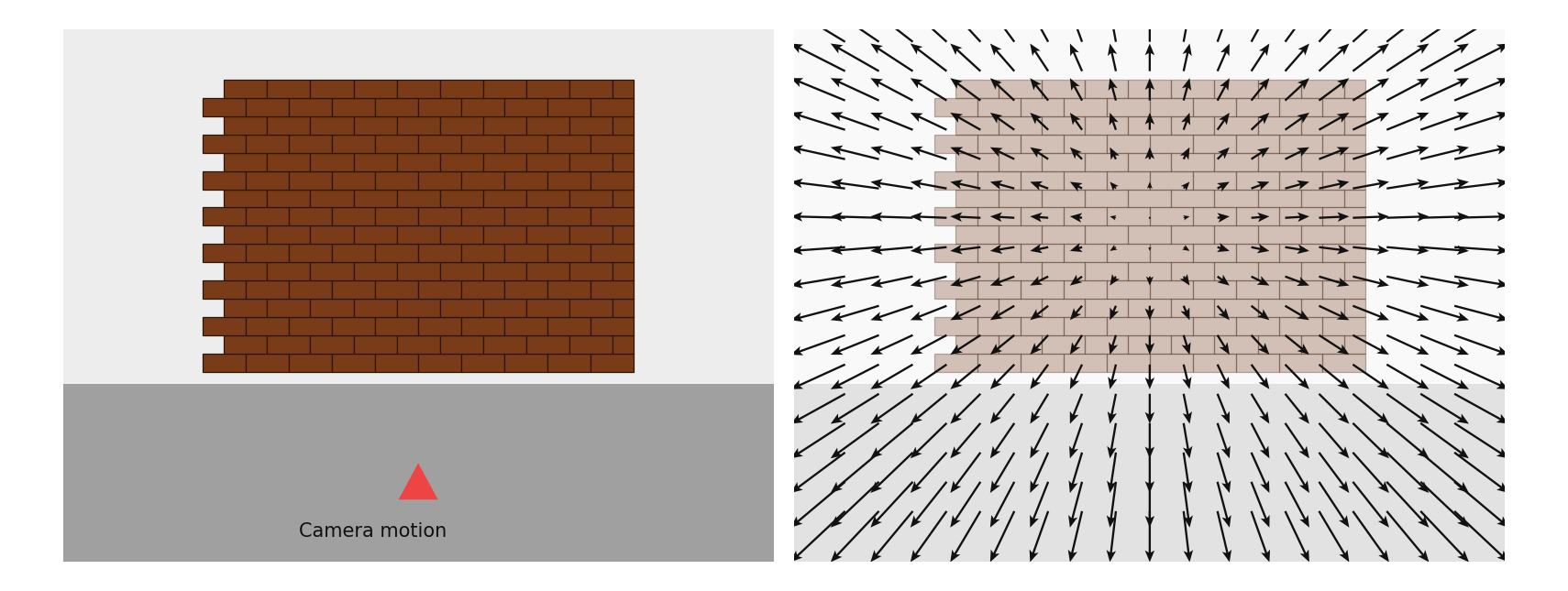
Forward camera motion and the focus of expansion

Driving toward a wall:

V_X = V_Y = 0

V_Z > 0

. Equation 47.5 simplifies to

\dot x = \frac{V_Z}{Z}\,x, \qquad \dot y = \frac{V_Z}{Z}\,y,

a radial flow centered at the origin. The point at which the field is zero is the focus of expansion, and the scaling factor

V_Z / Z

is the inverse time-to-contact, the quantity a fly’s-eye control loop reads off to time a landing.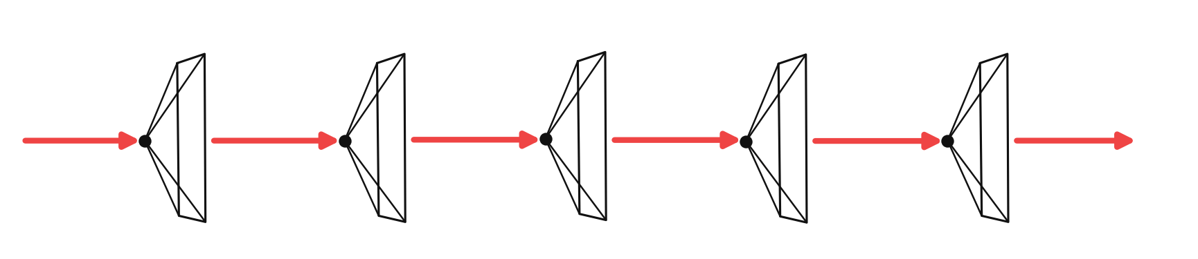

Camera rotation and the full motion field

Adding rotation, the point’s velocity relative to a rotating camera with angular velocity

\mathbf{\Omega}

\dot{\mathbf{P}} = -\mathbf{V} - \mathbf{\Omega} \times \mathbf{P}.

Plugging this into equation 47.1 produces the full motion field (equation 47.8):

\begin{bmatrix}\dot x\\\dot y\end{bmatrix} = \underbrace{\frac{1}{Z}\begin{bmatrix}-f & 0 & x\\0 & -f & y\end{bmatrix}\begin{bmatrix}V_X\\V_Y\\V_Z\end{bmatrix}}_{\text{translation: depends on }Z} \;+\; \underbrace{\frac{1}{f}\begin{bmatrix}xy & -(f^2+x^2) & fy\\ f^2+y^2 & -xy & -fx\end{bmatrix}\begin{bmatrix}\Omega_X\\\Omega_Y\\\Omega_Z\end{bmatrix}}_{\text{rotation: independent of }Z}.

Two qualitative consequences are worth noting:

Rotational flow is independent of depth, so it tells you nothing about the scene’s 3D structure.
Translational flow scales as $1/Z$ , so it carries all the depth information.

Figure 47.8 introduces the three rotation axes (yaw, pitch, roll) used throughout the rest of the chapter.

Rotation around the optical axis ( $\Omega_X = \Omega_Y = 0$ )

With only

\Omega_Z

active, equation 47.8 collapses to

\dot x = \Omega_Z\,y,\qquad \dot y = -\Omega_Z\,x,

the velocity field of rigid rotation about the image origin. Every concentric circle is an integral curve (figure 47.9).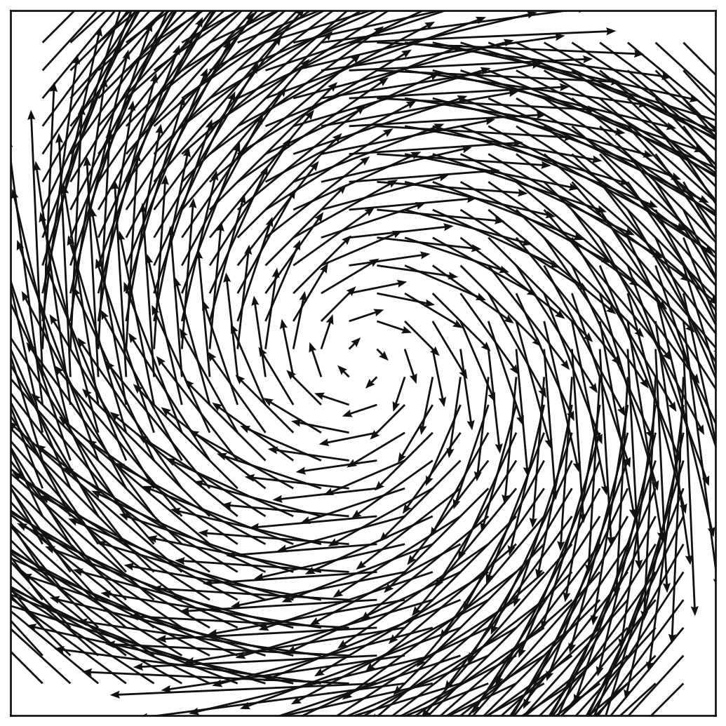

Rotation under varying focal length

Y-axis rotation with

\Omega_X = \Omega_Z = 0

produces

\dot x = -\frac{(f^2 + x^2)}{f}\,\Omega_Y,\qquad \dot y = -\frac{xy}{f}\,\Omega_Y,

which depends strongly on

f

. Wide-angle lenses (

f

small) produce flows with sharp curvature near the edges; long lenses (

f

large) produce nearly uniform horizontal flow. Figure 47.10 sweeps

f \in \{1/3, 1, 3\}

with the same scene and angular velocity.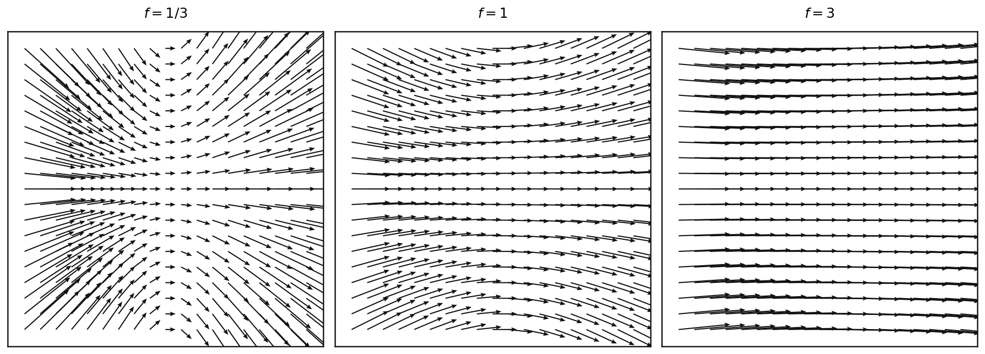

Concluding remarks

The whole chapter rests on three ideas:

Differentiate the projection $\mathbf{p} = (fX/Z, fY/Z)$ to get the image-plane motion of any moving 3D point (eq. 47.1).
Substitute the camera’s rigid-body kinematics $\dot{\mathbf{P}} = -\mathbf{V} - \mathbf{\Omega}\times\mathbf{P}$ to get the motion field (eq. 47.8).
Read off special cases: vanishing points (47.4), depth-modulated parallax (47.5), focus of expansion and time-to-contact (47.6), depth-independent rotation (47.7), focal-length sensitivity (47.10).

The next chapter of the book (48, optical flow) flips the script: given two frames, recover the motion field. The geometry here is the forward model that chapter inverts.

Edit this page on GitHub or file an issue.

Physical AI

3D Reconstruction

Imitation Learning

World Models

VLA Models

Sim-to-Real Transfer

3D Motion and Its 2D Projection

Perspective projection of a moving point

Two easy cases of equation 47.1

The vanishing point

The motion field under camera translation

Lateral camera motion

Forward camera motion and the focus of expansion

Camera rotation and the full motion field

Rotation around the optical axis ( $\Omega_X = \Omega_Y = 0$ )

Rotation under varying focal length

Concluding remarks

​Perspective projection of a moving point

​Two easy cases of equation 47.1

​The vanishing point

​The motion field under camera translation

​Lateral camera motion

​Forward camera motion and the focus of expansion

​Camera rotation and the full motion field

​Rotation around the optical axis (ΩX=ΩY=0\Omega_X = \Omega_Y = 0ΩX​=ΩY​=0)

​Rotation under varying focal length

​Concluding remarks

Perspective projection of a moving point

Two easy cases of equation 47.1

The vanishing point

The motion field under camera translation

Lateral camera motion

Forward camera motion and the focus of expansion

Camera rotation and the full motion field

Rotation around the optical axis ( $\Omega_X = \Omega_Y = 0$ )

Rotation under varying focal length

Concluding remarks