Estimating Motion by Patch Matching

This section was written by Ruimeng Yang (pull request #48), with help from an AI coding agent on the code. It reproduces the ideas of Chapter 46 of Foundations of Computer Vision by Antonio Torralba, Phillip Isola, and William T. Freeman. The book’s own figures are not reproduced here, because the book’s license covers only the work in full; links point to them instead. Motion estimation asks a simple question: if something moves between two frames, can you recover where it went? In this section you:

build intuition for motion in image coordinates,
recover motion with a readable patch-matching baseline,
estimate a sparse motion field on synthetic data with known ground truth,
measure accuracy with endpoint error and match ratios,
study how patch size, search radius, and noise change the results,
and inspect failure modes such as repetitive texture and motion that is too large.

The book’s figures

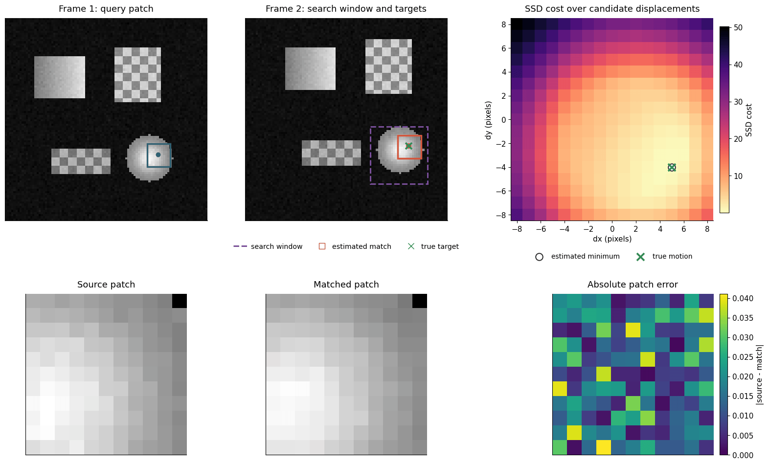
The book introduces the task with two frames of a street in Palma (Figure 46.3): each region of the first frame has to be assigned a displacement into the second. The code in this section solves the same task on synthetic frames with known ground truth. Related figures in the book:

the matching-cost map, whose minimum SSD location becomes the estimated displacement, the counterpart of the patch-matching diagnostic below;
the patch-size comparison: small patches are noisy, large patches blur motion boundaries, the same tradeoff the parameter sweep measures;
the perception demonstrations: a still photograph that implies motion, a static pattern that looks like it moves, and two space-time illusions (first, second);
the learned alternatives in chapter 49 of the book: a network that maps two frames directly to optical flow, and one that keeps features, a cost volume, and cost aggregation. The endpoint error that this section reports is defined there as well.

Intuition

Between two video frames, a moving object often keeps a similar local appearance. So a small patch around a point in Frame 1 may reappear a few pixels away in Frame 2. This section uses the image-coordinate convention common in vision:

$x$ increases to the right,
$y$ increases downward,
a motion vector is written as $(dx, dy)$ .

(dx=5, dy=-4)

means “move 5 pixels right and 4 pixels up.” The first figure below is generated from the synthetic frames used throughout the section. It marks three landmarks: the source patch in Frame 1, the true target in Frame 2, and the estimated target recovered by local patch matching. Because the example uses a known translation, you can check that the visual displacement and the recovered motion agree exactly.

import time
from pathlib import Path

import numpy as np
import matplotlib.pyplot as plt
from matplotlib.patches import FancyArrowPatch, Rectangle

rng = np.random.default_rng(7)

Synthetic example setup

Start with clean synthetic frames, because the true motion is known exactly. That lets you debug the estimator before dealing with real video. The scene uses a few textured geometric shapes so patch matching has enough visual structure to lock onto. The helper below builds a frame pair with a known integer translation. The motion-intuition figure comes later, once the patch matcher has also produced the estimated target.

def normalize_image(img):
    return np.clip(img, 0.0, 1.0)


def add_rectangle(img, x0, y0, w, h, base=0.75, texture="flat"):
    yy, xx = np.mgrid[y0 : y0 + h, x0 : x0 + w]
    patch = np.full((h, w), base, dtype=float)
    if texture == "gradient":
        patch *= 0.55 + 0.45 * (xx - x0) / max(w - 1, 1)
    elif texture == "checker":
        patch *= 0.65 + 0.35 * (((xx - x0) // 4 + (yy - y0) // 4) % 2)
    img[y0 : y0 + h, x0 : x0 + w] = np.maximum(img[y0 : y0 + h, x0 : x0 + w], patch)


def add_disk(img, cx, cy, radius, base=0.82):
    yy, xx = np.mgrid[: img.shape[0], : img.shape[1]]
    dist = np.sqrt((xx - cx) ** 2 + (yy - cy) ** 2)
    mask = dist <= radius
    ripple = 0.78 + 0.22 * np.cos(dist[mask] / max(radius, 1) * np.pi)
    img[mask] = np.maximum(img[mask], base * ripple)


def shift_image_integer(img, dx, dy, fill_value=0.06):
    shifted = np.full_like(img, fill_value)
    h, w = img.shape

    src_x0 = max(0, -dx)
    src_x1 = min(w, w - dx)
    src_y0 = max(0, -dy)
    src_y1 = min(h, h - dy)

    dst_x0 = max(0, dx)
    dst_x1 = dst_x0 + (src_x1 - src_x0)
    dst_y0 = max(0, dy)
    dst_y1 = dst_y0 + (src_y1 - src_y0)

    if src_x1 > src_x0 and src_y1 > src_y0:
        shifted[dst_y0:dst_y1, dst_x0:dst_x1] = img[src_y0:src_y1, src_x0:src_x1]
    return shifted


def make_synthetic_pair(dx=5, dy=-4, noise_std=0.0, size=96, seed=None):
    frame1 = np.full((size, size), 0.06, dtype=float)
    add_rectangle(frame1, 14, 18, 24, 20, base=0.88, texture="gradient")
    add_rectangle(frame1, 52, 14, 22, 26, base=0.82, texture="checker")
    add_rectangle(frame1, 22, 62, 28, 12, base=0.70, texture="checker")
    add_disk(frame1, 68, 66, 11, base=0.95)

    frame2 = shift_image_integer(frame1, dx=dx, dy=dy, fill_value=0.06)

    local_rng = np.random.default_rng(seed) if seed is not None else rng
    if noise_std > 0:
        frame1 = normalize_image(frame1 + local_rng.normal(0.0, noise_std, frame1.shape))
        frame2 = normalize_image(frame2 + local_rng.normal(0.0, noise_std, frame2.shape))

    return frame1, frame2, np.array([dx, dy], dtype=int)


def motion_to_index(dx, dy, search_radius):
    return dx + search_radius, dy + search_radius

demo_point_xy = (72, 64)
demo_patch_size = 11
frame1, frame2, gt_motion = make_synthetic_pair(dx=5, dy=-4, noise_std=0.015, seed=7)
demo_match = None

Patch matching by local search

The baseline method is deliberately simple:

extract an odd-sized patch around a point in Frame 1,
search a square window around the same location in Frame 2,
score each candidate with SSD (sum of squared differences),
keep the displacement with the lowest score.

It is easy to read and easy to reason about, which makes it a good baseline. The diagnostic figure below shows the whole loop in one place: source patch, searched region, SSD surface, matched patch, and patch error. The next cell defines helpers for patch extraction, SSD scoring, and exhaustive local search.

def extract_patch(image, center_xy, patch_size):
    radius = patch_size // 2
    x, y = map(int, center_xy)
    if x - radius < 0 or y - radius < 0:
        return None
    if x + radius >= image.shape[1] or y + radius >= image.shape[0]:
        return None
    return image[y - radius : y + radius + 1, x - radius : x + radius + 1]


def ssd_cost(template, candidate):
    diff = template - candidate
    return float(np.sum(diff * diff))


def filter_trackable_points(points, image_shape, patch_size, search_radius):
    radius = patch_size // 2 + search_radius
    height, width = image_shape
    valid_points = []
    for x, y in points:
        if radius <= x < width - radius and radius <= y < height - radius:
            valid_points.append((x, y))
    return valid_points


def estimate_patch_motion(frame1, frame2, point_xy, patch_size=11, search_radius=8):
    template = extract_patch(frame1, point_xy, patch_size)
    if template is None:
        raise ValueError("Source patch falls outside the image.")

    costs = np.full((2 * search_radius + 1, 2 * search_radius + 1), np.inf)
    best = {"cost": np.inf, "dx": 0, "dy": 0, "match_patch": None, "best_point": point_xy}

    for row, dy in enumerate(range(-search_radius, search_radius + 1)):
        for col, dx in enumerate(range(-search_radius, search_radius + 1)):
            candidate_point = (point_xy[0] + dx, point_xy[1] + dy)
            candidate = extract_patch(frame2, candidate_point, patch_size)
            if candidate is None:
                continue
            cost = ssd_cost(template, candidate)
            costs[row, col] = cost
            if cost < best["cost"]:
                best = {
                    "cost": cost,
                    "dx": dx,
                    "dy": dy,
                    "match_patch": candidate,
                    "best_point": candidate_point,
                }

    best["template_patch"] = template
    best["cost_map"] = costs
    return best

Single-point motion estimation

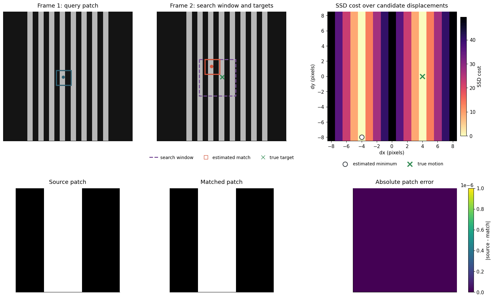
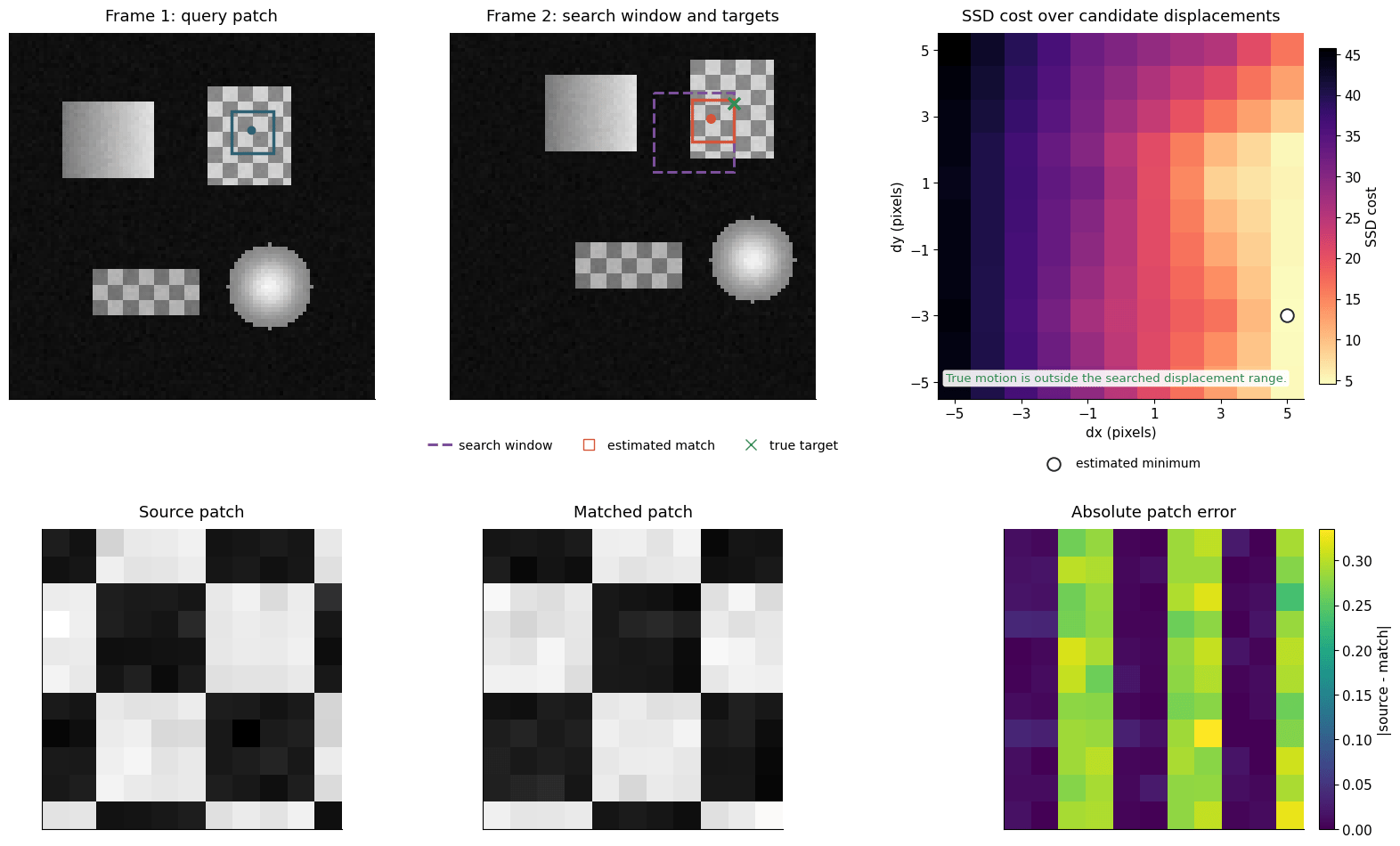
First, track one carefully chosen point so every part of the process is visible. Read the top row from left to right: the source patch in Frame 1, the searched region in Frame 2, and the SSD surface over candidate

(dx, dy)

displacements. Then compare the bottom-row patches: a low-error match means the winning displacement is also visually plausible.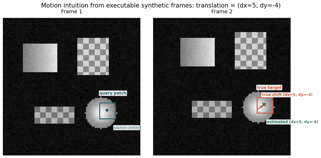

point_xy = demo_point_xy
patch_size = demo_patch_size
search_radius = 8

match_result = estimate_patch_motion(frame1, frame2, point_xy, patch_size=patch_size, search_radius=search_radius)
print(f"Estimated motion at {point_xy}: (dx={match_result['dx']}, dy={match_result['dy']})")
print(f"Ground truth motion: {tuple(map(int, gt_motion))}")
print(f"Best SSD cost: {match_result['cost']:.4f}")

Estimated motion at (72, 64): (dx=5, dy=-4)
Ground truth motion: (5, -4)
Best SSD cost: 0.0436

Single-point patch matching: estimated = (5, -4), true = (5, -4), best SSD = 0.0436

Sparse motion field estimation

One point builds intuition, but a motion field needs many arrows. You sample textured points on a grid, run the same local matcher at each one, and compute metrics over all valid points. To keep the figure readable, it shows only a subset of arrows, and exact estimates and mismatches are styled differently so the coherent global translation stands out.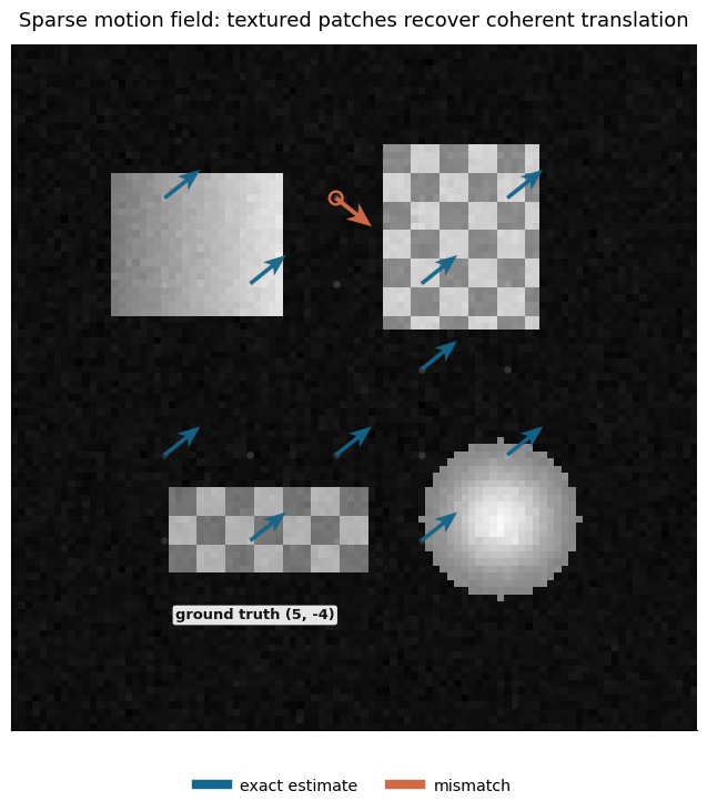

def sample_textured_points(frame, patch_size, stride=12, threshold=0.18):
    radius = patch_size // 2
    points = []
    for y in range(radius + 2, frame.shape[0] - radius - 2, stride):
        for x in range(radius + 2, frame.shape[1] - radius - 2, stride):
            patch = extract_patch(frame, (x, y), patch_size)
            if patch is None:
                continue
            if patch.std() > threshold or patch.mean() > 0.35:
                points.append((x, y))
    return points


def estimate_sparse_motion(frame1, frame2, points, patch_size=11, search_radius=8):
    estimates = []
    for point in points:
        result = estimate_patch_motion(frame1, frame2, point, patch_size=patch_size, search_radius=search_radius)
        estimates.append({
            "point": point,
            "dx": result["dx"],
            "dy": result["dy"],
            "cost": result["cost"],
        })
    return estimates


def summarize_motion_metrics(estimates, gt_motion):
    vectors = np.array([[item["dx"], item["dy"]] for item in estimates], dtype=float)
    gt = np.asarray(gt_motion, dtype=float)
    errors = vectors - gt[None, :]
    epe = np.sqrt(np.sum(errors ** 2, axis=1))
    exact = np.all(vectors == gt[None, :], axis=1)
    near = epe <= 1.0
    return {
        "num_points": len(estimates),
        "mean_epe": float(epe.mean()),
        "median_epe": float(np.median(epe)),
        "max_epe": float(epe.max()),
        "exact_match_ratio": float(exact.mean()),
        "within_1px_ratio": float(near.mean()),
    }

field_patch_size = 15
field_threshold = 0.08
candidate_points = sample_textured_points(frame1, patch_size=field_patch_size, stride=12, threshold=field_threshold)
points = filter_trackable_points(candidate_points, frame1.shape, patch_size=field_patch_size, search_radius=8)
estimates = estimate_sparse_motion(frame1, frame2, points, patch_size=field_patch_size, search_radius=8)
summary = summarize_motion_metrics(estimates, gt_motion)

print(
    f"Sparse field summary: {summary['num_points']} points, exact = {summary['exact_match_ratio']:.2f}, "
    f"within 1 px = {summary['within_1px_ratio']:.2f}, mean EPE = {summary['mean_epe']:.2f} px"
)

Sparse field summary: 22 points, exact = 0.95, within 1 px = 0.95, mean EPE = 0.36 px

Validation metrics

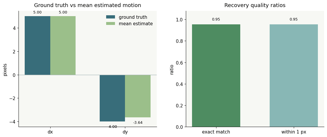
Because the synthetic translation is known, you can score the estimates directly.

Endpoint error (EPE) is the Euclidean distance between the estimated vector and the true vector.
Exact match ratio is the fraction of estimates that recover the exact integer motion.
Correct-within-1-pixel ratio is a softer measure that counts near misses as acceptable.

These metrics answer slightly different questions, so look at all of them. The printed summary reports the mean EPE explicitly.

metric_names = ["mean_epe", "median_epe", "max_epe", "exact_match_ratio", "within_1px_ratio"]
for key in metric_names:
    print(f"{key:>20}: {summary[key]:.3f}")

            mean_epe: 0.364
          median_epe: 0.000
             max_epe: 8.000
   exact_match_ratio: 0.955
    within_1px_ratio: 0.955

Metrics summary mean EPE: 0.36 px

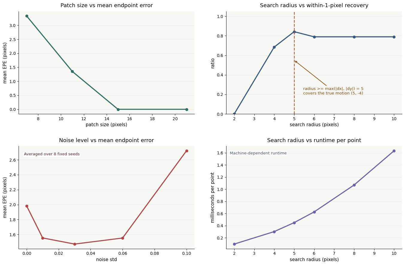
Parameter sweeps

Three knobs matter immediately:

Patch size: larger patches are often more stable, but they blur away local detail.
Search radius: larger windows can recover larger motion, but they cost more and may invite distractors.
Noise level: noisy images reduce the reliability of appearance matching.

The sweeps below come from controlled synthetic experiments. Because the true motion is

(5, -4)

, the search-radius plot also shows when the window first becomes large enough to contain the correct answer. The noise sweep averages over several fixed seeds, so the trend is not an artifact of one noisy draw.

def evaluate_setting(dx=5, dy=-4, noise_std=0.015, patch_size=11, search_radius=8, seed=123):
    f1, f2, gt = make_synthetic_pair(dx=dx, dy=dy, noise_std=noise_std, seed=seed)
    base_points = sample_textured_points(f1, patch_size=11, stride=12, threshold=0.08)
    points = filter_trackable_points(base_points, f1.shape, patch_size=patch_size, search_radius=search_radius)
    start = time.perf_counter()
    est = estimate_sparse_motion(f1, f2, points, patch_size=patch_size, search_radius=search_radius)
    elapsed_ms = 1000.0 * (time.perf_counter() - start)
    summary = summarize_motion_metrics(est, gt)
    summary["ms_per_point"] = elapsed_ms / max(len(points), 1)
    summary["num_points"] = len(points)
    return summary


patch_sizes = [7, 11, 15, 21]
search_radii = [2, 4, 5, 6, 8, 10]
noise_levels = [0.00, 0.01, 0.03, 0.06, 0.10]
noise_seeds = [101, 202, 303, 404, 505, 606, 707, 808]
required_radius = max(abs(int(gt_motion[0])), abs(int(gt_motion[1])))

patch_results = [evaluate_setting(patch_size=p, search_radius=8, noise_std=0.015, seed=321) for p in patch_sizes]
radius_results = [evaluate_setting(patch_size=11, search_radius=r, noise_std=0.015, seed=321) for r in search_radii]
noise_results = []
for noise_std in noise_levels:
    per_seed = [evaluate_setting(patch_size=11, search_radius=8, noise_std=noise_std, seed=seed) for seed in noise_seeds]
    noise_results.append(
        {
            "noise_std": noise_std,
            "mean_epe": float(np.mean([item["mean_epe"] for item in per_seed])),
            "within_1px_ratio": float(np.mean([item["within_1px_ratio"] for item in per_seed])),
        }
    )

Failure cases

A basic local matcher has clear blind spots. Two of the most important:

Repetitive texture: many candidate patches look equally good.
Motion outside the search radius: the correct answer is never even evaluated.

Both panels use the same ingredients as the successful single-point demo. What changes is the geometry of the problem: either the cost surface becomes ambiguous, or the true motion falls outside the searched range. The large-motion panel labels the true target as outside the searched region, so the wrong match is a limit of the search, not a bug in the plot.

def make_repetitive_texture_pair(dx=4, dy=0, size=96):
    frame1 = np.full((size, size), 0.08, dtype=float)
    for x0 in range(18, 78, 8):
        frame1[:, x0 : x0 + 4] = 0.72
    frame2 = shift_image_integer(frame1, dx=dx, dy=dy, fill_value=0.08)
    return frame1, frame2, np.array([dx, dy], dtype=int)

Failure A: repetitive texture ambiguity: estimated = (-4, -8), true = (4, 0), best SSD = 0.0000

Repeated stripes create nearly identical candidate patches at several displacements, so the SSD minimum is ambiguous even when the true motion lies inside the search window.
Failure B: motion beyond the search radius: estimated = (5, -3), true = (11, -7), best SSD = 4.5418
True target is outside the searched region, so patch matching cannot recover it.

The true target is outside the searched region, so patch matching cannot recover it and instead returns the best in-range candidate.

Limitations

Patch matching works well when:

motion is moderate,
the search window covers the true displacement,
local texture is distinctive,
and noise is not too strong.

It struggles when texture is ambiguous, motion is too large, illumination changes, or the motion varies strongly inside one patch. These limitations are why more advanced methods exist: Lucas-Kanade, Horn-Schunck optical flow, pyramidal search, and learned flow estimators. As an exercise, replace the global translation with a rotation or a locally varying motion and see where the baseline breaks first.

Edit this page on GitHub or file an issue.

Physical AI

3D Reconstruction

Imitation Learning

World Models

VLA Models

Sim-to-Real Transfer

Estimating Motion by Patch Matching

The book’s figures

Intuition

Synthetic example setup

Patch matching by local search

Single-point motion estimation

Sparse motion field estimation

Validation metrics

Parameter sweeps

Failure cases

Limitations

​The book’s figures

​Intuition

​Synthetic example setup

​Patch matching by local search

​Single-point motion estimation

​Sparse motion field estimation

​Validation metrics

​Parameter sweeps

​Failure cases

​Limitations

The book’s figures

Intuition

Synthetic example setup

Patch matching by local search

Single-point motion estimation

Sparse motion field estimation

Validation metrics

Parameter sweeps

Failure cases

Limitations