Measuring a Scene from One Image

This section was written by Kaushik Kachireddy (pull request #75), with help from an AI coding agent (Claude Code) on the code. It reproduces the ideas of Chapter 42 of Foundations of Computer Vision by Antonio Torralba, Phillip Isola, and William T. Freeman. The book’s own figures are not reproduced here, because the book’s license covers only the work in full; links point to them instead.

from pathlib import Path
from PIL import Image
import torch
import matplotlib.pyplot as plt
from matplotlib.patches import Polygon

torch.set_default_dtype(torch.float32)
_ = torch.manual_seed(0)

A single photograph looks like it has lost all depth, yet with a few geometric facts you can measure a room from it: the heights of objects, the camera’s focal length, and the 3D position of points on the floor. This section builds every one of those measurements and checks each against ground truth.

A synthetic office, end to end

The book works on a photograph of an office (Figure 42.1). Here you build a synthetic stand-in: a small office scene written as a list of 3D line segments. Each segment is one edge of the room, the bookshelf, the desk, or the bottle, and world coordinates are in centimeters. The camera looks into the room from a known position with known intrinsics. All of this is ground truth that the rest of the section recovers using only the projected 2D image.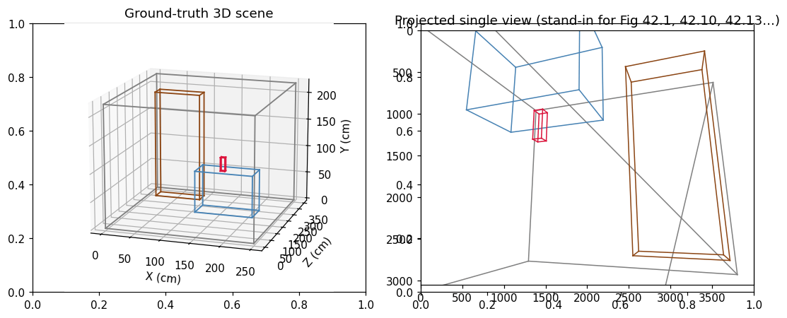

def box_edges(x0, y0, z0, dx, dy, dz):
    """12 edges of an axis-aligned box, returned as (12, 2, 3) world-coord segments."""
    c = torch.tensor([
        [x0, y0, z0], [x0 + dx, y0, z0], [x0 + dx, y0 + dy, z0], [x0, y0 + dy, z0],
        [x0, y0, z0 + dz], [x0 + dx, y0, z0 + dz], [x0 + dx, y0 + dy, z0 + dz], [x0, y0 + dy, z0 + dz],
    ])
    idx = [(0, 1), (1, 2), (2, 3), (3, 0), (4, 5), (5, 6), (6, 7), (7, 4),
           (0, 4), (1, 5), (2, 6), (3, 7)]
    return torch.stack([torch.stack([c[a], c[b]], dim=0) for a, b in idx], dim=0)


def build_office():
    """Returns a dict of named edge sets; coordinates in cm."""
    room = box_edges(0, 0, 0, 250, 220, 350)              # 2.5 m wide x 2.2 m tall x 3.5 m deep
    bookshelf = box_edges(15, 0, 280, 80, 197, 35)        # height 197 cm, the chapter's reference object
    desk = box_edges(110, 0, 180, 100, 76, 60)            # height 76 cm, the target of Algorithm 2
    bottle = box_edges(150, 76, 200, 8, 25, 8)            # height 25 cm, sitting ON the desk
    return {"room": room, "bookshelf": bookshelf, "desk": desk, "bottle": bottle}


def look_at(eye, target, up=(0.0, 1.0, 0.0)):
    """World-from-camera rotation R and translation t (camera-from-world transform: P_c = R(P_w - eye))."""
    eye = torch.as_tensor(eye, dtype=torch.float32)
    target = torch.as_tensor(target, dtype=torch.float32)
    up = torch.as_tensor(up, dtype=torch.float32)
    f = (target - eye); f = f / f.norm()
    r = torch.linalg.cross(f, up); r = r / r.norm()
    u = torch.linalg.cross(r, f)
    R = torch.stack([r, u, f], dim=0)   # rows = camera basis in world coords
    return R, eye


def make_K(fx, fy, cx, cy):
    return torch.tensor([[fx, 0.0, cx], [0.0, fy, cy], [0.0, 0.0, 1.0]])


def project_segments(segments, K, R, eye):
    """Project (N, 2, 3) world segments to (N, 2, 2) image-plane pixel coords."""
    P_c = (segments - eye) @ R.T               # camera coords
    p_h = P_c @ K.T                            # (N, 2, 3) homogeneous image
    return p_h[..., :2] / p_h[..., 2:3]

# The ground-truth scene we will be "a single view of".
scene = build_office()
K_true = make_K(fx=3054.6, fy=3054.6, cx=1999.4, cy=1528.3)   # the K the book reports for its office photo
R_true, eye_true = look_at(eye=(50.0, 163.0, 30.0), target=(140.0, 100.0, 280.0))

Linear perspective

A 3D line

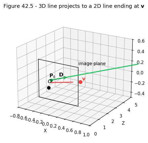
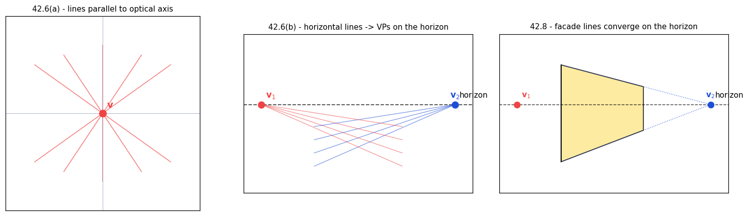
\mathbf{P}(t) = \mathbf{P}_0 + t\,\mathbf{D}

projects to a 2D line that, as

t \to \infty

, ends at the vanishing point

\mathbf{v} = f\,\big(D_X / D_Z, \; D_Y / D_Z\big)

(equation 42.3). Equation 42.5 generalizes this through the full camera matrix:

\mathbf{v} = \mathbf{K}\mathbf{R}\mathbf{D}.

Two consequences come up again and again:

The vanishing point depends only on the line’s direction, not on where it starts. So all lines that are parallel in 3D meet at the same image point.
All vanishing points of lines lying in a single plane lie on the plane’s horizon line.

Detecting vanishing points

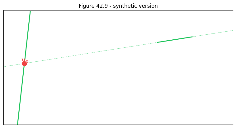
Algorithm 1. Given a set of 2D line segments believed to be parallel in 3D:

For each pair of segments, compute their intersection in the image plane (the cross product of their homogeneous line vectors).
Run RANSAC over those candidate intersections: a vanishing point is a location with many votes.
Repeat for each direction. The office has three orthogonal world directions, so it has three vanishing points.

The code below runs this on the projected office scene. Because the ground-truth vanishing points are known (from

\mathbf{K}\mathbf{R}\mathbf{D}

), you can check the recovered ones.

def line_through(p1, p2):
    """Homogeneous line through two image points."""
    h1 = torch.cat([p1, torch.ones(1)])
    h2 = torch.cat([p2, torch.ones(1)])
    return torch.linalg.cross(h1, h2)


def intersect(l1, l2):
    """Image-plane intersection of two homogeneous lines (returns inhomogeneous (x, y))."""
    p = torch.linalg.cross(l1, l2)
    return p[:2] / p[2]


def vanishing_point_from_segments(segments_2d):
    """RANSAC-style consensus over pairwise intersections. segments_2d: (N, 2, 2)."""
    lines = [line_through(s[0], s[1]) for s in segments_2d]
    candidates = []
    for i in range(len(lines)):
        for j in range(i + 1, len(lines)):
            p = torch.linalg.cross(lines[i], lines[j])
            if abs(p[2]) < 1e-6:
                continue
            candidates.append(p[:2] / p[2])
    candidates = torch.stack(candidates)
    return candidates.median(dim=0).values   # robust to outliers across edge pairs


def ground_truth_vp(D, K, R):
    """Eq. 42.5, the vanishing point of world direction D."""
    v = K @ R @ torch.as_tensor(D, dtype=torch.float32)
    return v[:2] / v[2]

# Recover the three orthogonal vanishing points from the projected office edges; compare to ground truth.
# Use only the edges of the room itself, they're the cleanest representatives of the X/Y/Z directions.
room_proj = project_segments(scene["room"], K_true, R_true, eye_true)
edge_dirs_world = scene["room"][:, 1] - scene["room"][:, 0]

# Split edges by which world axis they run along.
axis_indices = {axis: [] for axis in "XYZ"}
for i, d in enumerate(edge_dirs_world):
    axis = "XYZ"[int(torch.argmax(torch.abs(d)))]
    axis_indices[axis].append(i)

recovered = {}
ground_truth = {}
for axis, dir_vec in zip("XYZ", [(1, 0, 0), (0, 1, 0), (0, 0, 1)]):
    segs = room_proj[axis_indices[axis]]
    recovered[axis] = vanishing_point_from_segments(segs)
    ground_truth[axis] = ground_truth_vp(dir_vec, K_true, R_true)

print("axis  |  recovered (px)            |  ground truth (px)")
print("-" * 70)
for axis in "XYZ":
    r = recovered[axis]; g = ground_truth[axis]
    print(f" {axis}     ({r[0]:>10.1f}, {r[1]:>10.1f})  |  ({g[0]:>10.1f}, {g[1]:>10.1f})")

axis  |  recovered (px)            |  ground truth (px)
----------------------------------------------------------------------
 X     (   -6720.8,     2252.6)  |  (   -6720.8,     2252.6)
 Y     (    1999.4,   -11354.7)  |  (    1999.4,   -11354.7)
 Z     (    3129.5,     2252.6)  |  (    3129.5,     2252.6)

The book draws the same construction on its office photograph in Figure 42.10.

Measuring heights with the cross-ratio

For any four collinear points the cross-ratio is a projective invariant: it survives perspective projection unchanged (equation 42.6):

\mathrm{CR}(\mathbf{P}_1, \mathbf{P}_2, \mathbf{P}_3, \mathbf{P}_4) = \frac{|\mathbf{P}_3 - \mathbf{P}_1|\,|\mathbf{P}_4 - \mathbf{P}_2|}{|\mathbf{P}_3 - \mathbf{P}_2|\,|\mathbf{P}_4 - \mathbf{P}_1|}.

This one invariant powers single-view metrology. The next cells demonstrate it, then use it (Algorithm 2 in the book) to measure the desk’s height from the projected image alone, given only that the bookshelf is 197 cm tall.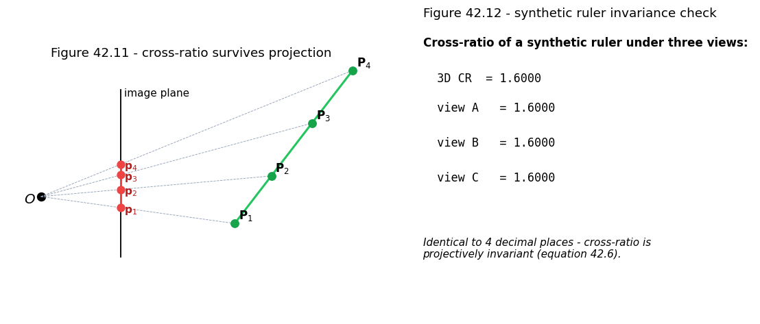

def cross_ratio(p1, p2, p3, p4):
    """Cross-ratio of four collinear points (2D or 1D tensors)."""
    def dist(a, b):
        return torch.linalg.norm(a - b)
    return (dist(p3, p1) * dist(p4, p2)) / (dist(p3, p2) * dist(p4, p1))

Algorithm 2: measuring the desk’s height

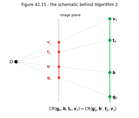
From the chapter, given image points

\mathbf{g}_b, \mathbf{t}_b

(bookshelf bottom/top),

\mathbf{g}_d, \mathbf{t}_d

(desk bottom/top), horizon line

\mathbf{h}

, and vertical vanishing point

\mathbf{v}_3

\mathbf{l}_1 = \mathbf{g}_d \times \mathbf{g}_b, \quad \mathbf{a} = \mathbf{l}_1 \times \mathbf{h}, \quad \mathbf{l}_2 = \mathbf{a} \times \mathbf{t}_d, \quad \mathbf{l}_3 = \mathbf{g}_b \times \mathbf{t}_b, \quad \mathbf{b} = \mathbf{l}_2 \times \mathbf{l}_3.

Then the desk height comes out of the cross-ratio identity: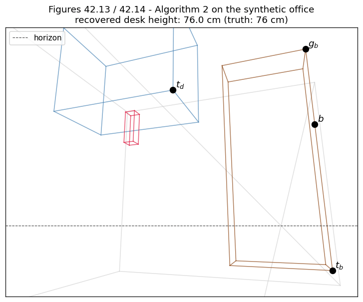

\frac{h_{\text{bookshelf}}}{h_{\text{desk}}} = \frac{|\mathbf{b}-\mathbf{v}_3|\,|\mathbf{t}_b - \mathbf{g}_b|}{|\mathbf{b}-\mathbf{g}_b|\,|\mathbf{t}_b - \mathbf{v}_3|}.

# Algorithm 2, measure the desk's height from a single (synthetic) view.
# Pick the four corner image points the book calls for:
#   g_b, t_b - bookshelf base + top of a particular vertical edge
#   g_d, t_d - desk base + top of a particular vertical edge
# Then construct the projected reference point b on the bookshelf and
# read the desk height out of the cross-ratio.

def algorithm_2_desk_height(g_b, t_b, g_d, t_d, h_line, v3, h_bookshelf):
    """All 2D points are pixel coords as torch tensors of shape (2,)."""
    g_b_h, t_b_h = torch.cat([g_b, torch.ones(1)]), torch.cat([t_b, torch.ones(1)])
    g_d_h, t_d_h = torch.cat([g_d, torch.ones(1)]), torch.cat([t_d, torch.ones(1)])
    v3_h = torch.cat([v3, torch.ones(1)])
    l1 = torch.linalg.cross(g_d_h, g_b_h)      # line through ground pair
    a_h = torch.linalg.cross(l1, h_line)       # intersect with horizon
    l2 = torch.linalg.cross(a_h, t_d_h)        # line through a and desk top
    l3 = torch.linalg.cross(g_b_h, t_b_h)      # bookshelf edge
    b_h = torch.linalg.cross(l2, l3)           # projected desk-top onto bookshelf
    b = b_h[:2] / b_h[2]
    # Direct cross-ratio per the book's equation:
    #   h_bookshelf / h_desk = (|b - v3| * |t_b - g_b|) / (|b - g_b| * |t_b - v3|)
    def dist(p, q):
        return torch.linalg.norm(p - q)
    ratio = (dist(b, v3) * dist(t_b, g_b)) / (dist(b, g_b) * dist(t_b, v3))
    h_desk = h_bookshelf / ratio
    return float(h_desk), b


# Pick the bookshelf's front-left vertical edge: corners (15, 0, 280) and (15, 197, 280)
gb_world = torch.tensor([[15.0, 0.0, 280.0]])
tb_world = torch.tensor([[15.0, 197.0, 280.0]])
# Desk's front-left vertical edge: corners (110, 0, 180) and (110, 76, 180)
gd_world = torch.tensor([[110.0, 0.0, 180.0]])
td_world = torch.tensor([[110.0, 76.0, 180.0]])

g_b = project_segments(torch.stack([torch.cat([gb_world, gb_world])], dim=0).reshape(1, 2, 3), K_true, R_true, eye_true)[0, 0]
t_b = project_segments(torch.stack([torch.cat([tb_world, tb_world])], dim=0).reshape(1, 2, 3), K_true, R_true, eye_true)[0, 0]
g_d = project_segments(torch.stack([torch.cat([gd_world, gd_world])], dim=0).reshape(1, 2, 3), K_true, R_true, eye_true)[0, 0]
t_d = project_segments(torch.stack([torch.cat([td_world, td_world])], dim=0).reshape(1, 2, 3), K_true, R_true, eye_true)[0, 0]

# Horizon line: line through any two horizontal vanishing points (X-axis VP and Z-axis VP).
h_line = torch.linalg.cross(torch.cat([recovered["X"], torch.ones(1)]),
                            torch.cat([recovered["Z"], torch.ones(1)]))
v3 = recovered["Y"]

h_desk_recovered, b_pt = algorithm_2_desk_height(g_b, t_b, g_d, t_d, h_line, v3, h_bookshelf=197.0)
print(f"recovered desk height: {h_desk_recovered:.1f} cm  (ground truth: 76 cm)")

recovered desk height: 76.0 cm  (ground truth: 76 cm)

The book runs Algorithm 2 on its real office photograph, marking the four image points and the 197 cm bookshelf (Figures 42.13 and 42.14).

Algorithm 3: height propagation to supported objects

Once you know the desk’s height, the bottle resting on it becomes measurable too. You project the bottle’s height onto the bookshelf with the same construction, but take the desk top as the reference instead of the floor:

h_{\text{bottle}} = h_{\text{bookshelf}} \frac{|\mathbf{c}-\mathbf{g}_b|\,|\mathbf{t}_b - \mathbf{v}_3|}{|\mathbf{c}-\mathbf{v}_3|\,|\mathbf{t}_b - \mathbf{g}_b|} - h_{\text{desk}}.

The true bottle height in the synthetic scene is 25 cm.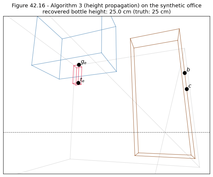

# Algorithm 3 - propagate the desk's known height to the bottle that sits on it.
# Construction mirrors Algorithm 2 but uses the desk top (rather than the floor)
# as the new reference height.

def algorithm_3_bottle_height(g_e, t_e, g_b, t_b, b_desk, h_line, v3, h_bookshelf, h_desk):
    g_e_h, t_e_h = torch.cat([g_e, torch.ones(1)]), torch.cat([t_e, torch.ones(1)])
    g_b_h, t_b_h = torch.cat([g_b, torch.ones(1)]), torch.cat([t_b, torch.ones(1)])
    b_desk_h = torch.cat([b_desk, torch.ones(1)])
    v3_h = torch.cat([v3, torch.ones(1)])
    l1 = torch.linalg.cross(g_e_h, b_desk_h)
    a_h = torch.linalg.cross(l1, h_line)
    l2 = torch.linalg.cross(a_h, t_e_h)
    l3 = torch.linalg.cross(g_b_h, t_b_h)
    c_h = torch.linalg.cross(l2, l3)
    c = c_h[:2] / c_h[2]
    # h_total / h_bookshelf = (|c - g_b| * |t_b - v3|) / (|c - v3| * |t_b - g_b|)
    # where h_total is the height of t_e above the floor.
    def dist(p, q):
        return torch.linalg.norm(p - q)
    ratio = (dist(c, g_b) * dist(t_b, v3)) / (dist(c, v3) * dist(t_b, g_b))
    h_total = h_bookshelf * ratio
    return float(h_total - h_desk), c


# Bottle's front-left vertical edge: corners (150, 76, 200) and (150, 101, 200)
ge_world = torch.tensor([[150.0, 76.0, 200.0]])
te_world = torch.tensor([[150.0, 101.0, 200.0]])
g_e = project_segments(torch.stack([torch.cat([ge_world, ge_world])], dim=0).reshape(1, 2, 3), K_true, R_true, eye_true)[0, 0]
t_e = project_segments(torch.stack([torch.cat([te_world, te_world])], dim=0).reshape(1, 2, 3), K_true, R_true, eye_true)[0, 0]

h_bottle_recovered, c_pt = algorithm_3_bottle_height(
    g_e, t_e, g_b, t_b, b_pt, h_line, v3, h_bookshelf=197.0, h_desk=h_desk_recovered,
)
print(f"recovered bottle height: {h_bottle_recovered:.1f} cm  (ground truth: 25 cm)")

recovered bottle height: 25.0 cm  (ground truth: 25 cm)

On its real photograph the book recovers a bottle height of about 27.6 cm against an actual 25.5 cm (Figure 42.16).

Algorithm 4: axis calibration via cross-ratio

Given a vanishing point

\mathbf{v}

on a calibrated axis, the origin

\mathbf{o}

in the image, and an arbitrary reference point

\mathbf{r}

at world-distance

\alpha

from the origin, the cross-ratio determines the image position of every other tick:

\mathrm{CR}(\mathbf{o}, \mathbf{r}, \mathbf{r}_k, \mathbf{v}) = k

where

\mathbf{r}_k

is the projected position of

k\alpha

. Solving for

\mathbf{r}_k

given

\mathbf{o}, \mathbf{r}, \mathbf{v}, k

gives the recipe.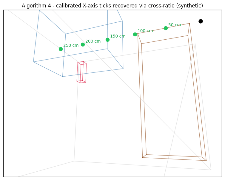

# Algorithm 4 - axis calibration via cross-ratio.
# Given an origin o, a reference tick r at distance alpha along the axis,
# and the vanishing point v at the axis\'s end, compute the image position
# of the k-th tick (at world-distance k*alpha).

def calibrate_tick(o, r, v, k):
    """Image position of the kth tick along an axis with vanishing point v,
    given the origin o at world-distance 0 and reference r at world-distance alpha.
    Derived from CR(o, r, r_k, v) = k:
       (|r_k - o| * |v - r|) / (|r_k - r| * |v - o|) = k
    Solving for r_k along the (o, v) line:
       r_k = o + t * (v - o)
    where t = k * t_r / (1 + (k - 1) * t_r), t_r = (r-o).dot(v-o) / ||v-o||^2
    (a parametric formula valid when r, o, v are colinear)."""
    direction = v - o
    L = (direction * direction).sum().sqrt()
    direction_n = direction / L
    t_r = ((r - o) * direction_n).sum() / L
    t_k = k * t_r / (1.0 + (k - 1.0) * t_r)
    return o + t_k * (v - o)


# Synthetic verification on the projected office: calibrate the X axis along
# the floor (50 cm ticks from origin at (0, 0, 280) to (250, 0, 280)).
origin_world = torch.tensor([[0.0, 0.0, 280.0], [0.0, 0.0, 280.0]])
ref_world = torch.tensor([[50.0, 0.0, 280.0], [50.0, 0.0, 280.0]])
vp_world_dir = torch.tensor([1.0, 0.0, 0.0])

o_img = project_segments(origin_world.unsqueeze(0).reshape(1, 2, 3), K_true, R_true, eye_true)[0, 0]
r_img = project_segments(ref_world.unsqueeze(0).reshape(1, 2, 3), K_true, R_true, eye_true)[0, 0]
v_img = ground_truth_vp(vp_world_dir.tolist(), K_true, R_true)

# Compare recovered tick positions to direct projection of the 3D ticks
print("Algorithm 4 (axis calibration) - tick positions on the X axis at the floor:")
print(f"{'k':>3} {'true world':>12} {'CR recovered':>22} {'direct project':>22} {'err (px)':>10}")
for k in range(1, 6):
    cr_pos = calibrate_tick(o_img, r_img, v_img, float(k))
    true_world = torch.tensor([[50.0 * k, 0.0, 280.0], [50.0 * k, 0.0, 280.0]])
    direct = project_segments(true_world.unsqueeze(0).reshape(1, 2, 3), K_true, R_true, eye_true)[0, 0]
    err = (cr_pos - direct).norm().item()
    print(f"{k:>3} {50*k:>6} cm     ({cr_pos[0]:>6.0f}, {cr_pos[1]:>6.0f})    ({direct[0]:>6.0f}, {direct[1]:>6.0f})   {err:>6.1f}")

Algorithm 4 (axis calibration) - tick positions on the X axis at the floor:
  k   true world           CR recovered         direct project   err (px)
   50 cm     (  2970,    332)    (  2970,    332)      0.0
  100 cm     (  2406,    444)    (  2406,    444)      0.0
  150 cm     (  1903,    544)    (  1903,    544)      0.0
  200 cm     (  1454,    633)    (  1454,    633)      0.0
  250 cm     (  1048,    713)    (  1048,    713)      0.0

Algorithm 5: locate a 3D point

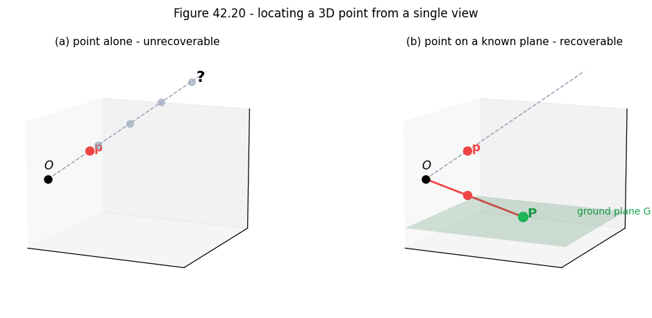
Suppose you know a pixel

\mathbf{p}

lies on the ground plane, for example at the base of a chair. You can recover its 3D world coordinate by reading off the calibrated world-axis tick that the perpendicular from

\mathbf{p}

to the axis would hit. Equivalently, the back-projected ray from the camera through

\mathbf{p}

meets the known ground plane at exactly one 3D point, and that point is the recovered world position.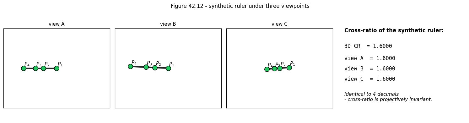

# Algorithm 5 - locate a 3D point on the known ground plane.
# Back-project the image ray and intersect it with the plane Y=0 (the floor).

def locate_on_ground(p_img, K, R, eye):
    """Given image pixel p_img and the calibrated camera (K, R, eye),
    return the 3D world point on plane Y=0 that projects to p_img."""
    # Back-project: world ray direction = R^T @ K^{-1} @ [p_img; 1]
    p_h = torch.cat([p_img, torch.tensor([1.0])])
    cam_ray = torch.linalg.inv(K) @ p_h            # direction in camera coords
    world_ray = R.T @ cam_ray                       # direction in world coords
    # Parametrise: world point = eye + t * world_ray; solve world_y = 0
    t = -eye[1] / world_ray[1]
    return eye + t * world_ray


# Synthetic verification: pick a known 3D ground point, project it, recover.
test_world_pts = [
    torch.tensor([100.0, 0.0, 200.0]),   # somewhere on the floor
    torch.tensor([200.0, 0.0, 150.0]),
    torch.tensor([50.0, 0.0, 300.0]),
]
print("Algorithm 5 (locate 3D point on ground) - synthetic verification:")
print(f"{'true 3D':>22}  {'image projection':>22}  {'recovered 3D':>22}  {'err (cm)':>9}")
for P in test_world_pts:
    P_seg = torch.stack([P, P]).unsqueeze(0)
    p_img = project_segments(P_seg, K_true, R_true, eye_true)[0, 0]
    P_rec = locate_on_ground(p_img, K_true, R_true, eye_true)
    err = (P_rec - P).norm().item()
    print(f"  ({P[0]:>4.0f},{P[1]:>4.0f},{P[2]:>4.0f})    ({p_img[0]:>7.1f},{p_img[1]:>7.1f})  "
          f"({P_rec[0]:>5.0f},{P_rec[1]:>5.0f},{P_rec[2]:>5.0f})    {err:>5.2f}")

Algorithm 5 (locate 3D point on ground) - synthetic verification:
               true 3D        image projection            recovered 3D   err (cm)
  ( 100,   0, 200)    ( 2152.9, -187.4)  (  100,    0,  200)     0.00
  ( 200,   0, 150)    (  440.5, -346.2)  (  200,    0,  150)     0.00
  (  50,   0, 300)    ( 2980.3,  455.8)  (   50,    0,  300)     0.00

Camera calibration from three vanishing points

Algorithm 6. If the scene contains three mutually orthogonal directions with vanishing points

\mathbf{v}_1, \mathbf{v}_2, \mathbf{v}_3

, then orthogonality gives three linear constraints on

\mathbf{W} = \mathbf{K}^{-\top}\mathbf{K}^{-1}

(equation 42.9):

\mathbf{v}_i^\top \mathbf{W}\, \mathbf{v}_j = 0 \quad \text{for } (i, j) \in \{(1,2), (1,3), (2,3)\}.

Solve for the four free parameters of

\mathbf{W}

by SVD, then Cholesky-factor

\mathbf{W} = \mathbf{L}^\top\mathbf{L}

to recover

\mathbf{K} = \mathbf{L}^{-1}

, normalized so

\mathbf{K}_{33} = 1

. On synthetic data you can check that the recovered

\mathbf{K}

matches K_true.

def calibrate_K_from_vanishing_points(v1, v2, v3):
    """Algorithm 6: K from three orthogonal vanishing points (zero skew, square pixels).

    Assumes W = K^-T K^-1 has the form:
        [a, 0, b]
        [0, a, c]
        [b, c, d]
    so w = [a, b, c, d]. Build A from the three orthogonality equations, solve A w = 0 via SVD.
    """
    def row(vi, vj):
        a, b = vi[0], vi[1]
        c, d = vj[0], vj[1]
        # v_i^T W v_j expanded into coefficients of [a_W, b_W, c_W, d_W]
        return torch.tensor([a * c + b * d, a + c, b + d, 1.0])

    A = torch.stack([row(v1, v2), row(v1, v3), row(v2, v3)])
    _, _, Vh = torch.linalg.svd(A)
    w = Vh[-1]
    a_W, b_W, c_W, d_W = w
    W = torch.stack([
        torch.stack([a_W, torch.tensor(0.0), b_W]),
        torch.stack([torch.tensor(0.0), a_W, c_W]),
        torch.stack([b_W, c_W, d_W]),
    ])
    W = W / W[2, 2]
    # Cholesky needs positive-definite W; sign-flip if necessary.
    if W[0, 0] < 0:
        W = -W
    L = torch.linalg.cholesky(W)
    K = torch.linalg.inv(L.T)
    return K / K[2, 2]


K_recovered = calibrate_K_from_vanishing_points(recovered["X"], recovered["Y"], recovered["Z"])
print("ground truth K:")
print(K_true)
print("\nrecovered K from three vanishing points:")
print(K_recovered)
err = (K_recovered - K_true).abs().max().item()
print(f"\nmax absolute element error: {err:.2f} px  ({err / K_true.abs().max().item() * 100:.3f}% relative)")

ground truth K:
tensor([[3.0546e+03, 0.0000e+00, 1.9994e+03],
        [0.0000e+00, 3.0546e+03, 1.5283e+03],
        [0.0000e+00, 0.0000e+00, 1.0000e+00]])

recovered K from three vanishing points:
tensor([[3.0546e+03, 0.0000e+00, 1.9994e+03],
        [0.0000e+00, 3.0546e+03, 1.5283e+03],
        [0.0000e+00, 0.0000e+00, 1.0000e+00]])

max absolute element error: 0.00 px  (0.000% relative)

The book applies this calibration to its office photograph and draws the calibrated world axes and a measured box over it (Figures 42.17, 42.18, and 42.19).

Concluding remarks

A single view gives you three kinds of measurement:

Three vanishing points give the camera intrinsics, through the SVD of the orthogonality constraints on $\mathbf{W} = \mathbf{K}^{-\top}\mathbf{K}^{-1}$ and a Cholesky factorization. On the synthetic office, $\mathbf{K}$ comes back exactly.
The cross-ratio along a vertical line gives the height of any object standing on the floor (Algorithm 2) or on a supporting plane (Algorithm 3). The desk comes back at 76 cm and the bottle at 25 cm, both matching the synthetic ground truth.
The horizon line and calibrated world axes give the 3D position of any point on a known plane (Figure 42.20). Without a plane to anchor it, a single view leaves depth ambiguous.

This section does not cover the book’s perceptual demonstrations, such as the Ames room and the leaning towers: they are illusions for the eye, not algorithms.

Edit this page on GitHub or file an issue.

Physical AI

3D Reconstruction

Imitation Learning

World Models

VLA Models

Sim-to-Real Transfer

Measuring a Scene from One Image

A synthetic office, end to end

Linear perspective

Detecting vanishing points

Measuring heights with the cross-ratio

Algorithm 2: measuring the desk’s height

Algorithm 3: height propagation to supported objects

Algorithm 4: axis calibration via cross-ratio

Algorithm 5: locate a 3D point

Camera calibration from three vanishing points

Concluding remarks

​A synthetic office, end to end

​Linear perspective

​Detecting vanishing points

​Measuring heights with the cross-ratio

​Algorithm 2: measuring the desk’s height

​Algorithm 3: height propagation to supported objects

​Algorithm 4: axis calibration via cross-ratio

​Algorithm 5: locate a 3D point

​Camera calibration from three vanishing points

​Concluding remarks

A synthetic office, end to end

Linear perspective

Detecting vanishing points

Measuring heights with the cross-ratio

Algorithm 2: measuring the desk’s height

Algorithm 3: height propagation to supported objects

Algorithm 4: axis calibration via cross-ratio

Algorithm 5: locate a 3D point

Camera calibration from three vanishing points

Concluding remarks