Homographies and Robust Estimation

This section was written by Ruimeng Yang (pull request #43), with help from an AI coding agent on the code. It reproduces the ideas of Chapter 41 of Foundations of Computer Vision by Antonio Torralba, Phillip Isola, and William T. Freeman. In this section you build a homography estimator from scratch in PyTorch, check it on synthetic point correspondences, see when it works and when it breaks, and finish by correcting the perspective of a synthetic image. By the end you should be able to:

explain what a planar homography does,
move between Euclidean and homogeneous coordinates,
estimate a homography with the normalized DLT algorithm,
measure reprojection error,
use RANSAC to reject outliers,
warp a planar image patch with inverse warping,
and recognize failure modes such as degenerate point sets and overwhelming outlier rates.

What a homography does

A homography is a

3 \times 3

matrix that maps points from one image plane to another. It describes the mapping exactly when the scene is planar, or when the camera only rotates about its optical center. This section stays deliberately narrow. It works on synthetic data so the geometry is easy to see, and it is not a panorama stitcher. The aim is to show how the math, the point correspondences, the robust estimation, and the final perspective correction fit together. You implement DLT, RANSAC, and inverse warping in PyTorch and use them to:

visualize how one plane is warped into another,
estimate a homography from noisy correspondences,
measure reprojection error,
reject outliers with RANSAC,
and rectify a synthetic checkerboard with inverse warping.

Throughout, the section moves back and forth between pictures and equations, so you can connect the matrix notation to something geometric.

Homogeneous coordinates and $\tilde{\mathbf{p}}' \sim H\tilde{\mathbf{p}}$

A 2D point

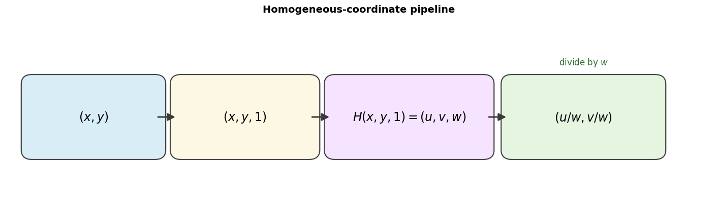
\mathbf{p} = (x, y)

becomes a homogeneous 3-vector by appending a 1:

\tilde{\mathbf{p}} = \begin{bmatrix}x \\ y \\ 1\end{bmatrix}.

A homography is a non-singular matrix

H \in \mathbb{R}^{3 \times 3}, \qquad \tilde{\mathbf{p}}' \sim H\tilde{\mathbf{p}}.

The symbol

\sim

means equal up to scale. In homogeneous coordinates, multiplying a point by any nonzero scalar does not change the represented Euclidean point. After applying

H

, you convert back to Euclidean coordinates by dividing by the last component:

\tilde{\mathbf{p}}' = \begin{bmatrix}u \\ v \\ w\end{bmatrix} \quad \Rightarrow \quad \mathbf{p}' = \left(\frac{u}{w}, \frac{v}{w}\right).

Because

H

is defined only up to a scale factor, compare estimated and ground-truth homographies after normalizing them to a common scale. A counting argument helps here. A homography is written as a 3x3 matrix, which suggests 9 entries, but multiplying the whole matrix by any nonzero constant gives the same geometric mapping. That means one overall scale is arbitrary, so the homography has 8 degrees of freedom, not 9. Each point correspondence contributes two constraints, one for the destination x-coordinate and one for the destination y-coordinate. Therefore four non-collinear point pairs are the minimum needed for DLT, while using more than four correspondences gives an overdetermined least-squares system. To estimate

H

from correspondences, you use the normalized Direct Linear Transform (DLT):

normalize source and destination points for numerical stability,
write the linear constraints implied by each correspondence,
solve the resulting homogeneous system with SVD,
denormalize the result back into the original coordinate system.

DLT also needs point configurations that constrain the full 2D projective warp. If all correspondences are collinear or nearly collinear, the system becomes poorly conditioned because the data do not sufficiently constrain the whole plane. The failure cases at the end of this section demonstrate that degeneracy. The implementation here does not filter degenerate samples, but production estimators often reject them before accepting a fit. The last coordinate

w

lets a matrix represent perspective effects, and dividing by

w

is the step that brings the transformed point back to ordinary 2D coordinates.

import math
import random
from pathlib import Path

import matplotlib.pyplot as plt
from matplotlib.patches import FancyArrowPatch, FancyBboxPatch, Polygon
import torch


torch.set_default_dtype(torch.float64)
_ = torch.manual_seed(7)
random.seed(7)

Synthetic data setup

You create a regular 2D grid of points, define a known homography, and use it to generate perfect correspondences. This gives a clean baseline before noise and outliers are added.

def to_homogeneous(points: torch.Tensor) -> torch.Tensor:
    """Append a 1 to each 2D point."""
    if points.ndim != 2 or points.shape[1] != 2:
        raise ValueError("Expected points with shape (N, 2).")
    ones = torch.ones((points.shape[0], 1), dtype=points.dtype, device=points.device)
    return torch.cat([points, ones], dim=1)


def from_homogeneous(points: torch.Tensor, eps: float = 1e-12) -> torch.Tensor:
    """Convert homogeneous points back to Euclidean coordinates."""
    if points.ndim != 2 or points.shape[1] != 3:
        raise ValueError("Expected homogeneous points with shape (N, 3).")
    scale = points[:, 2:].clone()
    scale = torch.where(scale.abs() < eps, torch.full_like(scale, eps), scale)
    return points[:, :2] / scale


def apply_homography(points: torch.Tensor, H: torch.Tensor) -> torch.Tensor:
    """Apply a 3x3 homography to 2D points."""
    if H.shape != (3, 3):
        raise ValueError("Expected H with shape (3, 3).")
    warped = to_homogeneous(points) @ H.T
    return from_homogeneous(warped)


def normalize_points(points: torch.Tensor, eps: float = 1e-12) -> tuple[torch.Tensor, torch.Tensor]:
    """Normalize points so the centroid is at the origin and mean distance is sqrt(2)."""
    centroid = points.mean(dim=0)
    centered = points - centroid
    mean_dist = torch.linalg.norm(centered, dim=1).mean().clamp(min=eps)
    scale = math.sqrt(2.0) / mean_dist

    T = torch.tensor(
        [
            [scale, 0.0, -scale * centroid[0]],
            [0.0, scale, -scale * centroid[1]],
            [0.0, 0.0, 1.0],
        ],
        dtype=points.dtype,
        device=points.device,
    )
    normalized = apply_homography(points, T)
    return normalized, T


def estimate_homography_dlt(src_points: torch.Tensor, dst_points: torch.Tensor) -> torch.Tensor:
    """Estimate a homography with normalized DLT."""
    if src_points.shape != dst_points.shape or src_points.shape[0] < 4:
        raise ValueError("Need at least four matching point pairs.")

    src_norm, T_src = normalize_points(src_points)
    dst_norm, T_dst = normalize_points(dst_points)

    rows = []
    for (x, y), (u, v) in zip(src_norm, dst_norm):
        rows.append(
            torch.tensor(
                [-x, -y, -1.0, 0.0, 0.0, 0.0, u * x, u * y, u],
                dtype=src_points.dtype,
                device=src_points.device,
            )
        )
        rows.append(
            torch.tensor(
                [0.0, 0.0, 0.0, -x, -y, -1.0, v * x, v * y, v],
                dtype=src_points.dtype,
                device=src_points.device,
            )
        )
    A = torch.stack(rows)

    _, _, vh = torch.linalg.svd(A)
    H_norm = vh[-1].reshape(3, 3)
    H = torch.linalg.inv(T_dst) @ H_norm @ T_src
    return H / torch.linalg.norm(H)


def compute_reprojection_error(H: torch.Tensor, src_points: torch.Tensor, dst_points: torch.Tensor) -> torch.Tensor:
    """Compute Euclidean reprojection error for each correspondence."""
    projected = apply_homography(src_points, H)
    return torch.linalg.norm(projected - dst_points, dim=1)


def ransac_homography(
    src_points: torch.Tensor,
    dst_points: torch.Tensor,
    threshold: float,
    num_iters: int,
) -> tuple[torch.Tensor, torch.Tensor, dict]:
    """Estimate a homography robustly with four-point RANSAC."""
    if src_points.shape[0] < 4:
        raise ValueError("RANSAC needs at least four correspondences.")

    n = src_points.shape[0]
    best_H = None
    best_inliers = None
    best_count = -1
    best_mean_error = float("inf")

    for _ in range(num_iters):
        sample_idx = torch.randperm(n)[:4]
        try:
            candidate_H = estimate_homography_dlt(src_points[sample_idx], dst_points[sample_idx])
        except RuntimeError:
            continue

        errors = compute_reprojection_error(candidate_H, src_points, dst_points)
        inliers = errors < threshold
        count = int(inliers.sum().item())
        mean_error = float(errors[inliers].mean().item()) if count > 0 else float("inf")

        if count > best_count or (count == best_count and mean_error < best_mean_error):
            best_H = candidate_H
            best_inliers = inliers
            best_count = count
            best_mean_error = mean_error

    if best_H is None or best_inliers is None or int(best_inliers.sum().item()) < 4:
        raise RuntimeError("RANSAC failed to find a valid homography.")

    refined_H = estimate_homography_dlt(src_points[best_inliers], dst_points[best_inliers])
    refined_errors = compute_reprojection_error(refined_H, src_points, dst_points)
    diagnostics = {
        "mean_inlier_error": float(refined_errors[best_inliers].mean().item()),
        "mean_all_error": float(refined_errors.mean().item()),
        "num_inliers": int(best_inliers.sum().item()),
        "inlier_ratio": float(best_inliers.double().mean().item()),
    }
    return refined_H, best_inliers, diagnostics


def normalize_homography_scale(H: torch.Tensor) -> torch.Tensor:
    """Normalize a homography so it can be compared up to scale."""
    if abs(float(H[-1, -1])) > 1e-12:
        return H / H[-1, -1]
    return H / torch.linalg.norm(H)


def make_grid(num_x: int = 6, num_y: int = 6, spacing: float = 1.0) -> torch.Tensor:
    xs = torch.linspace(-2.5, 2.5, steps=num_x) * spacing
    ys = torch.linspace(-2.0, 2.0, steps=num_y) * spacing
    yy, xx = torch.meshgrid(ys, xs, indexing="ij")
    return torch.stack([xx.reshape(-1), yy.reshape(-1)], dim=1)

src_grid = make_grid()
H_gt = torch.tensor(
    [
        [1.10, 0.18, 1.20],
        [-0.12, 0.95, -0.60],
        [0.015, 0.020, 1.00],
    ]
)

dst_grid_clean = apply_homography(src_grid, H_gt)
print("Number of correspondences:", src_grid.shape[0])
print("Ground-truth H:")
print(normalize_homography_scale(H_gt))

Number of correspondences: 36
Ground-truth H:
tensor([[ 1.1000,  0.1800,  1.2000],
        [-0.1200,  0.9500, -0.6000],
        [ 0.0150,  0.0200,  1.0000]])

Visualizing the known transformation

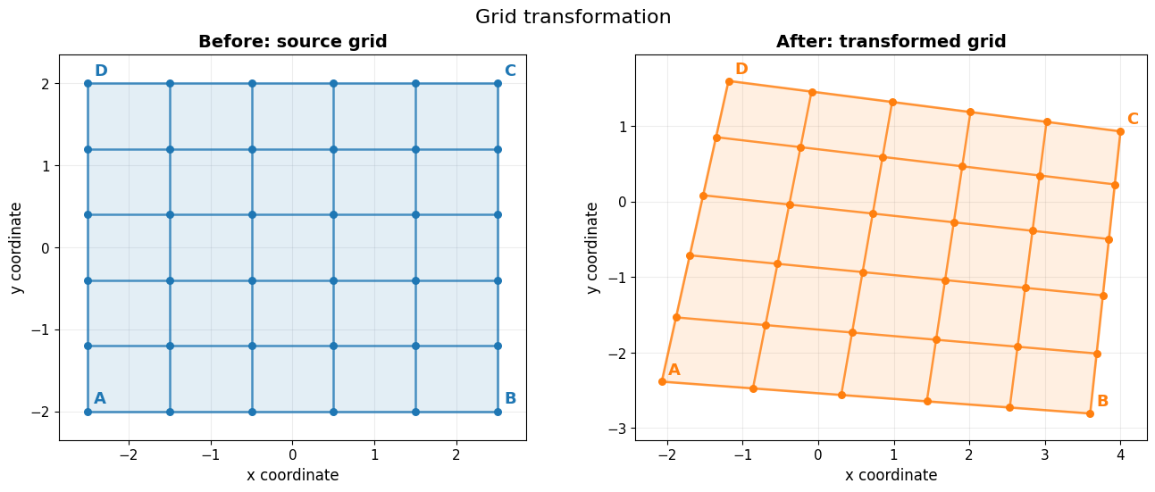
The next figures show a regular source grid on one plane and the warped grid on the destination plane. The first is the conceptual plane-to-plane view; the second is the literal before-and-after view of the same coordinates. A homography bends the square boundary into a quadrilateral while still preserving straight lines. Every source point stays on the same underlying plane, but perspective changes spacing, orientation, and apparent parallelism. DLT and RANSAC try to recover exactly this planar warp from noisy point matches. The labeled corners A, B, C, and D form a non-collinear quadrilateral. This is the geometric reason four non-collinear correspondences are the minimum for DLT: they are the smallest set that constrains a full planar projective warp rather than only a line-like slice of it.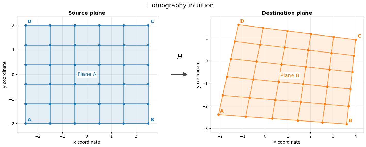

Noisy correspondences and outliers

Real feature matches are never perfect. You perturb the destination points with Gaussian noise and then replace a fraction of them with random outliers. This tests both least-squares estimation and robust estimation under controlled conditions. Some destination points stay close to the clean warp, while the outliers jump far away. A few bad matches are enough to damage a plain least-squares fit. The hard part is not only estimating a homography, but deciding which correspondences deserve to influence the estimate.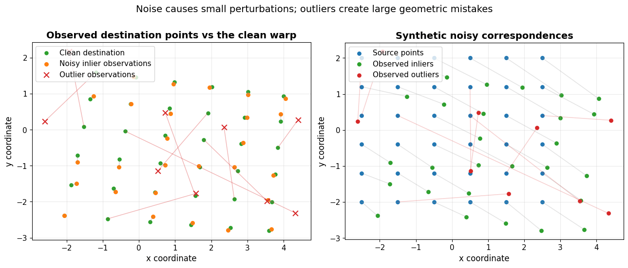

def generate_correspondences(
    H: torch.Tensor,
    noise_std: float = 0.05,
    outlier_ratio: float = 0.2,
    num_x: int = 6,
    num_y: int = 6,
) -> tuple[torch.Tensor, torch.Tensor, torch.Tensor, torch.Tensor]:
    src = make_grid(num_x=num_x, num_y=num_y)
    dst_clean = apply_homography(src, H)
    dst_noisy = dst_clean + noise_std * torch.randn_like(dst_clean)

    num_points = src.shape[0]
    num_outliers = int(round(outlier_ratio * num_points))
    true_inliers = torch.ones(num_points, dtype=torch.bool)

    if num_outliers > 0:
        outlier_idx = torch.randperm(num_points)[:num_outliers]
        mins = dst_clean.min(dim=0).values - 1.0
        maxs = dst_clean.max(dim=0).values + 1.0
        random_points = mins + (maxs - mins) * torch.rand((num_outliers, 2), dtype=dst_noisy.dtype)
        dst_noisy[outlier_idx] = random_points
        true_inliers[outlier_idx] = False

    return src, dst_clean, dst_noisy, true_inliers


src_points, dst_clean, dst_points, true_inliers = generate_correspondences(
    H_gt,
    noise_std=0.08,
    outlier_ratio=0.25,
)

print("True inlier ratio:", true_inliers.double().mean().item())

True inlier ratio: 0.75

Estimation: DLT versus RANSAC

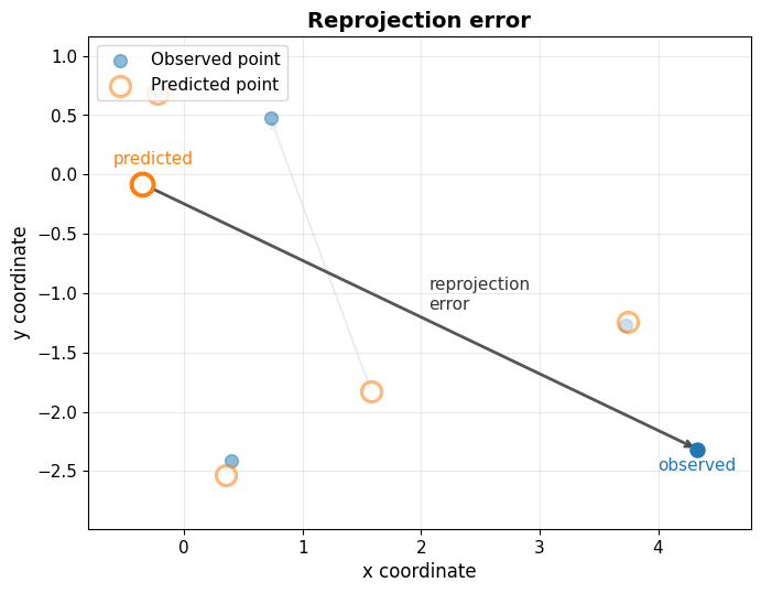
You first estimate a homography from all correspondences with normalized DLT. Then you run RANSAC: repeatedly sample four points, score each candidate by reprojection error, and refit on the best inlier set. The outputs below show the DLT pipeline, a plot of observed against predicted destination points that illustrates reprojection error, and a numerical comparison of plain DLT and RANSAC. DLT answers the question “which matrix best explains these equations?” RANSAC adds the question “which correspondences should you trust before solving those equations?” The SVD step recovers a normalized homography

H_{\text{norm}}

. You then map it back to the original coordinate system with

H = T_{\mathrm{dst}}^{-1} H_{\mathrm{norm}} T_{\mathrm{src}}.

This denormalization step is why point normalization improves numerical stability without changing the final geometric mapping.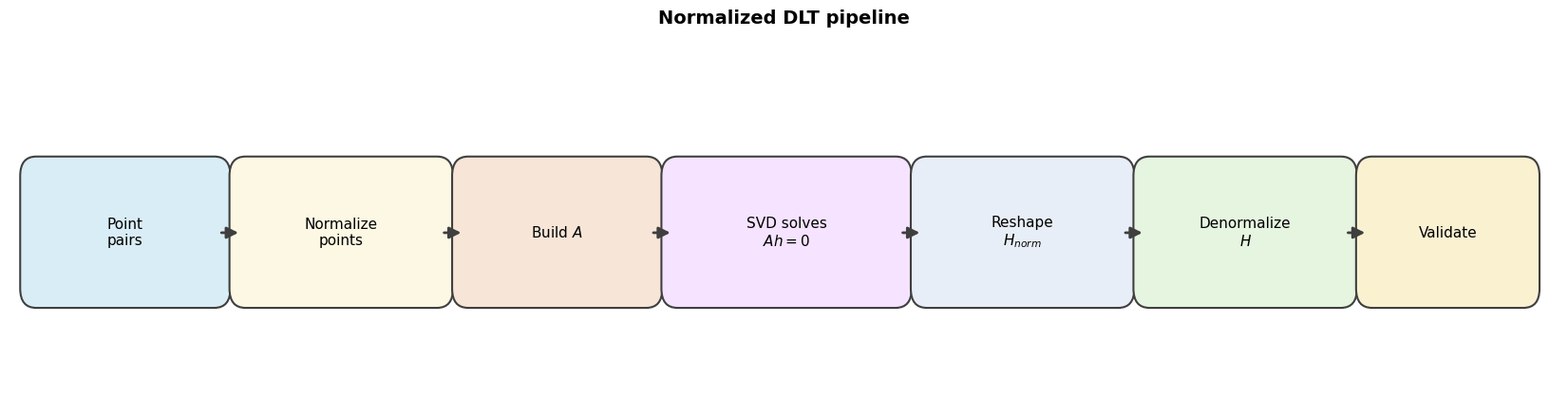

H_dlt = estimate_homography_dlt(src_points, dst_points)
errors_dlt = compute_reprojection_error(H_dlt, src_points, dst_points)

H_ransac, predicted_inliers, ransac_info = ransac_homography(
    src_points,
    dst_points,
    threshold=0.20,
    num_iters=400,
)
errors_ransac = compute_reprojection_error(H_ransac, src_points, dst_points)
projected_ransac = apply_homography(src_points, H_ransac)

selected_idx = torch.tensor([2, 9, 17, 25, int(torch.argmax(errors_ransac).item())], dtype=torch.long)
observed_small = dst_points[selected_idx]
predicted_small = projected_ransac[selected_idx]
error_small = errors_ransac[selected_idx]
highlight_local = int(torch.argmax(error_small).item())
highlight_global = int(selected_idx[highlight_local].item())

print("DLT mean reprojection error:   ", float(errors_dlt.mean().item()))
print("RANSAC mean reprojection error:", float(errors_ransac.mean().item()))
print("RANSAC diagnostics:", ransac_info)
print("Highlighted reprojection pair index:", highlight_global)

DLT mean reprojection error:    1.0240097483168158
RANSAC mean reprojection error: 0.6730099428317433
RANSAC diagnostics: {'mean_inlier_error': 0.08344928815809421, 'mean_all_error': 0.6730099428317433, 'num_inliers': 25, 'inlier_ratio': 0.6944444444444444}
Highlighted reprojection pair index: 19

RANSAC inliers and outliers

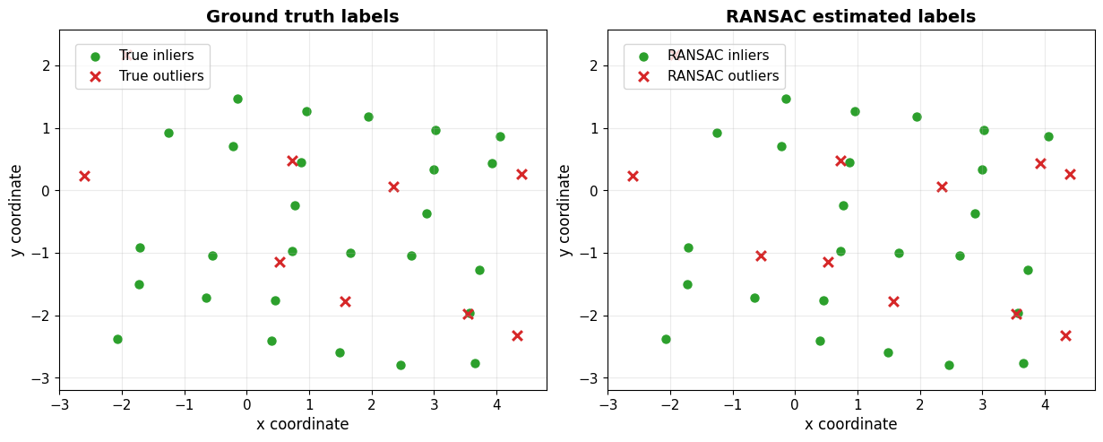
The next plot colors the matched destination points by whether RANSAC classified them as inliers or outliers. The left panel is the synthetic ground-truth split and the right panel is RANSAC’s estimate, on the same axes. RANSAC does not try to explain every point. It looks for the largest self-consistent subset of matches and ignores the points that break that consistency. Once the inliers are identified, the homography is refit using only those correspondences.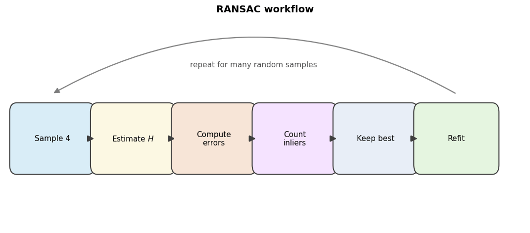

Validation against ground truth

A homography is only defined up to scale, so the estimated and true matrices are normalized before they are compared. Three kinds of metrics are reported:

Frobenius matrix error: how far the estimated homography is from the ground truth after scale normalization,
mean reprojection error: the average Euclidean mismatch between predicted and observed destination points,
RANSAC precision and recall: how accurately the robust estimator separated true inliers from outliers.

Lower matrix and reprojection errors are better; higher precision and recall are better. Reprojection error tells you whether the estimated geometry lands in the right place, while precision and recall tell you whether RANSAC trusted the right correspondences.

H_gt_scaled = normalize_homography_scale(H_gt)
H_dlt_scaled = normalize_homography_scale(H_dlt)
H_ransac_scaled = normalize_homography_scale(H_ransac)

matrix_error_dlt = torch.linalg.norm(H_gt_scaled - H_dlt_scaled).item()
matrix_error_ransac = torch.linalg.norm(H_gt_scaled - H_ransac_scaled).item()
mean_reproj_error = errors_ransac.mean().item()
inlier_ratio = predicted_inliers.double().mean().item()
precision = (predicted_inliers & true_inliers).sum().item() / max(predicted_inliers.sum().item(), 1)
recall = (predicted_inliers & true_inliers).sum().item() / max(true_inliers.sum().item(), 1)

print("Ground-truth H (normalized):")
print(H_gt_scaled)
print()
print("DLT estimate (normalized):")
print(H_dlt_scaled)
print()
print("RANSAC estimate (normalized):")
print(H_ransac_scaled)
print()
print("Frobenius error vs ground truth (lower is better)")
print("  DLT:   ", matrix_error_dlt)
print("  RANSAC:", matrix_error_ransac)
print()
print("Mean reprojection error over all correspondences:", mean_reproj_error)
print("RANSAC predicted inlier ratio:              ", inlier_ratio)
print("RANSAC precision:                           ", precision)
print("RANSAC recall:                              ", recall)

Ground-truth H (normalized):
tensor([[ 1.1000,  0.1800,  1.2000],
        [-0.1200,  0.9500, -0.6000],
        [ 0.0150,  0.0200,  1.0000]])

DLT estimate (normalized):
tensor([[ 1.3546,  0.0878,  1.7850],
        [-0.1269,  1.0427, -0.6914],
        [ 0.1299, -0.0290,  1.0000]])

RANSAC estimate (normalized):
tensor([[ 1.0924,  0.1661,  1.2214],
        [-0.1167,  0.9399, -0.6258],
        [ 0.0175,  0.0133,  1.0000]])

Frobenius error vs ground truth (lower is better)
  DLT:    0.6694519651771217
  RANSAC: 0.03922417890699948

Mean reprojection error over all correspondences: 0.6730099428317433
RANSAC predicted inlier ratio:               0.6944444444444444
RANSAC precision:                            1.0
RANSAC recall:                               0.9259259259259259

Perspective correction with inverse warping

A homography moves more than sparse points. Once you know the mapping between two views of the same plane, you can move every pixel on that plane. This makes homographies useful for rectification: undoing a perspective distortion so the plane looks fronto-parallel again. You create a synthetic checkerboard, warp it with a known homography, and rectify it with inverse warping. The figure compares the original, distorted, and rectified views. Dense warping needs interpolation, because inverse-mapped coordinates usually land between integer pixel locations.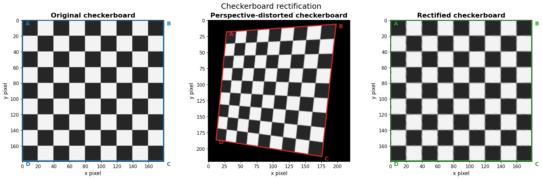

def create_checkerboard(
    height: int = 180,
    width: int = 180,
    num_checks_x: int = 9,
    num_checks_y: int = 9,
) -> torch.Tensor:
    """Create a grayscale checkerboard image with values in [0, 1]."""
    y = torch.arange(height, dtype=torch.get_default_dtype())
    x = torch.arange(width, dtype=torch.get_default_dtype())
    yy, xx = torch.meshgrid(y, x, indexing="ij")

    check_x = torch.clamp((xx * num_checks_x / width).floor().long(), max=num_checks_x - 1)
    check_y = torch.clamp((yy * num_checks_y / height).floor().long(), max=num_checks_y - 1)
    board = ((check_x + check_y) % 2).to(torch.get_default_dtype())
    return 0.15 + 0.8 * board


def bilinear_interpolate(image: torch.Tensor, x: torch.Tensor, y: torch.Tensor) -> tuple[torch.Tensor, torch.Tensor]:
    """Sample an image at floating-point coordinates with bilinear interpolation."""
    if image.ndim == 2:
        image_3d = image.unsqueeze(-1)
        squeeze_channel = True
    elif image.ndim == 3:
        image_3d = image
        squeeze_channel = False
    else:
        raise ValueError("Expected image with shape (H, W) or (H, W, C).")

    height, width, _ = image_3d.shape
    x0 = torch.floor(x).long()
    y0 = torch.floor(y).long()
    x1 = x0 + 1
    y1 = y0 + 1

    valid = (x >= 0.0) & (x <= width - 1) & (y >= 0.0) & (y <= height - 1)

    x0c = x0.clamp(0, width - 1)
    x1c = x1.clamp(0, width - 1)
    y0c = y0.clamp(0, height - 1)
    y1c = y1.clamp(0, height - 1)

    Ia = image_3d[y0c, x0c]
    Ib = image_3d[y0c, x1c]
    Ic = image_3d[y1c, x0c]
    Id = image_3d[y1c, x1c]

    x0f = x0.to(image_3d.dtype)
    x1f = x1.to(image_3d.dtype)
    y0f = y0.to(image_3d.dtype)
    y1f = y1.to(image_3d.dtype)

    wa = (x1f - x) * (y1f - y)
    wb = (x - x0f) * (y1f - y)
    wc = (x1f - x) * (y - y0f)
    wd = (x - x0f) * (y - y0f)

    sampled = (
        wa.unsqueeze(-1) * Ia
        + wb.unsqueeze(-1) * Ib
        + wc.unsqueeze(-1) * Ic
        + wd.unsqueeze(-1) * Id
    )
    sampled = sampled * valid.unsqueeze(-1)

    if squeeze_channel:
        sampled = sampled.squeeze(-1)
    return sampled, valid


def inverse_warp_image(
    image: torch.Tensor,
    H_src_from_dst: torch.Tensor,
    out_height: int,
    out_width: int,
) -> tuple[torch.Tensor, torch.Tensor]:
    """Warp an image by inverse mapping from destination pixels to source pixels."""
    y = torch.arange(out_height, dtype=image.dtype)
    x = torch.arange(out_width, dtype=image.dtype)
    yy, xx = torch.meshgrid(y, x, indexing="ij")

    dst_points = torch.stack([xx.reshape(-1), yy.reshape(-1)], dim=1)
    src_points = apply_homography(dst_points, H_src_from_dst)

    sampled, valid = bilinear_interpolate(image, src_points[:, 0], src_points[:, 1])
    if image.ndim == 2:
        warped = sampled.reshape(out_height, out_width)
    else:
        warped = sampled.reshape(out_height, out_width, image.shape[2])
    return warped, valid.reshape(out_height, out_width)


checkerboard = create_checkerboard()
board_height, board_width = checkerboard.shape

src_corners = torch.tensor(
    [
        [0.0, 0.0],
        [board_width - 1.0, 0.0],
        [board_width - 1.0, board_height - 1.0],
        [0.0, board_height - 1.0],
    ]
)

dst_corners = torch.tensor(
    [
        [28.0, 18.0],
        [198.0, 6.0],
        [176.0, 212.0],
        [12.0, 186.0],
    ]
)

H_checkerboard = estimate_homography_dlt(src_corners, dst_corners)
distorted_checkerboard, distorted_mask = inverse_warp_image(
    checkerboard,
    torch.linalg.inv(H_checkerboard),
    out_height=220,
    out_width=220,
)
rectified_checkerboard, rectified_mask = inverse_warp_image(
    distorted_checkerboard,
    H_checkerboard,
    out_height=board_height,
    out_width=board_width,
)

print("Checkerboard homography (normalized):")
print(normalize_homography_scale(H_checkerboard))
print("Distorted coverage ratio:", float(distorted_mask.double().mean().item()))
print("Rectified coverage ratio:", float(rectified_mask.double().mean().item()))

Checkerboard homography (normalized):
tensor([[ 7.4405e-01, -8.8605e-02,  2.8000e+01],
        [-7.3272e-02,  9.5065e-01,  1.8000e+01],
        [-1.0387e-03,  6.5044e-05,  1.0000e+00]])
Distorted coverage ratio: 0.6478512396694215
Rectified coverage ratio: 1.0

rectification_mae = (rectified_checkerboard[rectified_mask] - checkerboard[rectified_mask]).abs().mean().item()
print(f"Rectification mean absolute error over valid rectified pixels: {rectification_mae:.4f}")

Rectification mean absolute error over valid rectified pixels: 0.0294

Bilinear interpolation is needed because inverse-mapped source coordinates are almost never integers. A destination pixel often lands between four source pixels, so you blend those neighbors instead of rounding to the nearest one. This avoids staircase artifacts. The rectified board is fronto-parallel again, but interpolation slightly softens the edges. The example is idealized: the checkerboard is perfectly planar, the four corner correspondences are noise-free, and there is no lens distortion, occlusion, or lighting change. The rectification error is therefore mainly a resampling artifact from interpolating twice. Real photographs add many more complications.

Parameter study

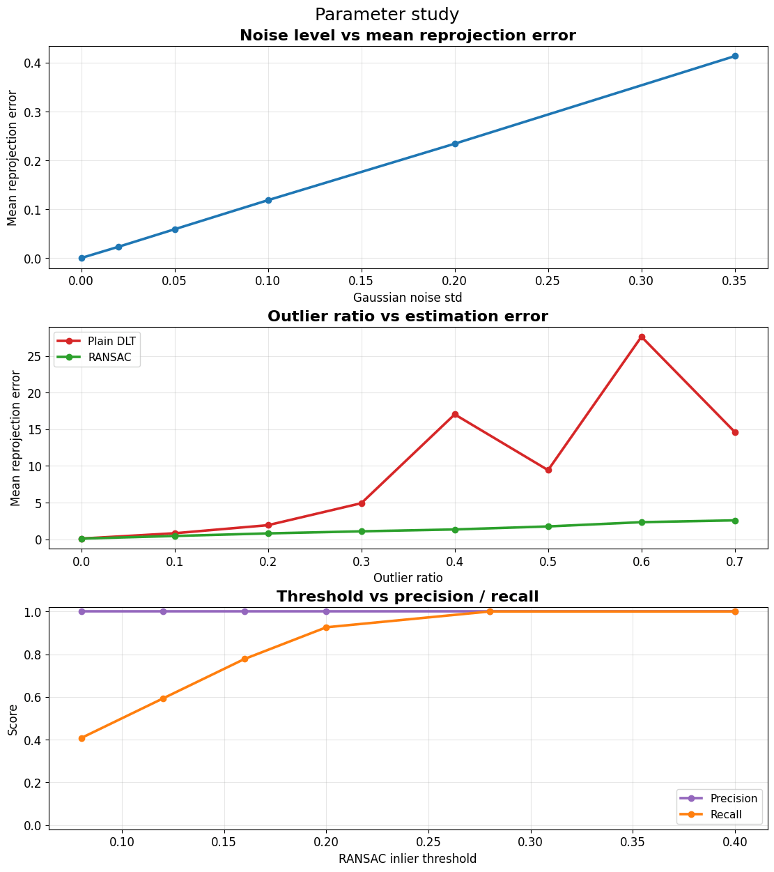
Two practical questions matter:

How does measurement noise affect reprojection error?
How do outliers and the inlier threshold affect robust estimation?

The next experiment sweeps over both.

noise_levels = [0.0, 0.02, 0.05, 0.10, 0.20, 0.35]
noise_errors = []

for noise_std in noise_levels:
    trial_errors = []
    for _ in range(20):
        src, _, dst, _ = generate_correspondences(H_gt, noise_std=noise_std, outlier_ratio=0.0)
        H_est = estimate_homography_dlt(src, dst)
        trial_errors.append(compute_reprojection_error(H_est, src, dst).mean().item())
    noise_errors.append(sum(trial_errors) / len(trial_errors))

outlier_ratios = [0.0, 0.10, 0.20, 0.30, 0.40, 0.50, 0.60, 0.70]
dlt_reproj_errors = []
ransac_reproj_errors = []

for outlier_ratio in outlier_ratios:
    dlt_trials = []
    ransac_trials = []
    for _ in range(20):
        src, _, dst, _ = generate_correspondences(H_gt, noise_std=0.08, outlier_ratio=outlier_ratio)
        H_dlt_trial = estimate_homography_dlt(src, dst)
        dlt_trials.append(compute_reprojection_error(H_dlt_trial, src, dst).mean().item())
        try:
            H_est, _, _ = ransac_homography(src, dst, threshold=0.20, num_iters=500)
            ransac_trials.append(compute_reprojection_error(H_est, src, dst).mean().item())
        except RuntimeError:
            pass
    dlt_reproj_errors.append(sum(dlt_trials) / len(dlt_trials))
    ransac_reproj_errors.append(sum(ransac_trials) / len(ransac_trials) if ransac_trials else float("nan"))

thresholds = [0.08, 0.12, 0.16, 0.20, 0.28, 0.40]
threshold_precisions = []
threshold_recalls = []
for threshold in thresholds:
    try:
        _, inliers_t, _ = ransac_homography(src_points, dst_points, threshold=threshold, num_iters=400)
        tp = int((inliers_t & true_inliers).sum().item())
        precision_t = tp / max(int(inliers_t.sum().item()), 1)
        recall_t = tp / max(int(true_inliers.sum().item()), 1)
    except RuntimeError:
        precision_t = 0.0
        recall_t = 0.0
    threshold_precisions.append(precision_t)
    threshold_recalls.append(recall_t)

for noise_std, err in zip(noise_levels, noise_errors):
    print(f"noise_std={noise_std:>4.2f} -> mean error={err:.4f}")
print()
for outlier_ratio, dlt_err, ransac_err in zip(outlier_ratios, dlt_reproj_errors, ransac_reproj_errors):
    print(f"outlier_ratio={outlier_ratio:>4.2f} -> DLT mean error={dlt_err:.3f}, RANSAC mean error={ransac_err:.3f}")
print()
for threshold, precision_t, recall_t in zip(thresholds, threshold_precisions, threshold_recalls):
    print(f"threshold={threshold:>4.2f} -> precision={precision_t:.2f}, recall={recall_t:.2f}")

noise_std=0.00 -> mean error=0.0000
noise_std=0.02 -> mean error=0.0230
noise_std=0.05 -> mean error=0.0588
noise_std=0.10 -> mean error=0.1184
noise_std=0.20 -> mean error=0.2340
noise_std=0.35 -> mean error=0.4133

outlier_ratio=0.00 -> DLT mean error=0.098, RANSAC mean error=0.099
outlier_ratio=0.10 -> DLT mean error=0.826, RANSAC mean error=0.454
outlier_ratio=0.20 -> DLT mean error=1.926, RANSAC mean error=0.807
outlier_ratio=0.30 -> DLT mean error=4.924, RANSAC mean error=1.088
outlier_ratio=0.40 -> DLT mean error=17.026, RANSAC mean error=1.345
outlier_ratio=0.50 -> DLT mean error=9.430, RANSAC mean error=1.755
outlier_ratio=0.60 -> DLT mean error=27.611, RANSAC mean error=2.336
outlier_ratio=0.70 -> DLT mean error=14.622, RANSAC mean error=2.585

threshold=0.08 -> precision=1.00, recall=0.41
threshold=0.12 -> precision=1.00, recall=0.59
threshold=0.16 -> precision=1.00, recall=0.78
threshold=0.20 -> precision=1.00, recall=0.93
threshold=0.28 -> precision=1.00, recall=1.00
threshold=0.40 -> precision=1.00, recall=1.00

Increasing noise weakens each correspondence, so reprojection error rises even when every match is correct. Increasing the outlier ratio makes plain DLT fragile, while RANSAC stays stable only as long as it can still find a consistent model. The inlier threshold is a tradeoff: too small rejects noisy but valid points, too large admits outliers. The first two panels plot a geometric error; the last plots precision and recall, which are unitless rates. Keeping them on separate axes avoids a misleading comparison.

Failure cases: degeneracy and extreme outliers

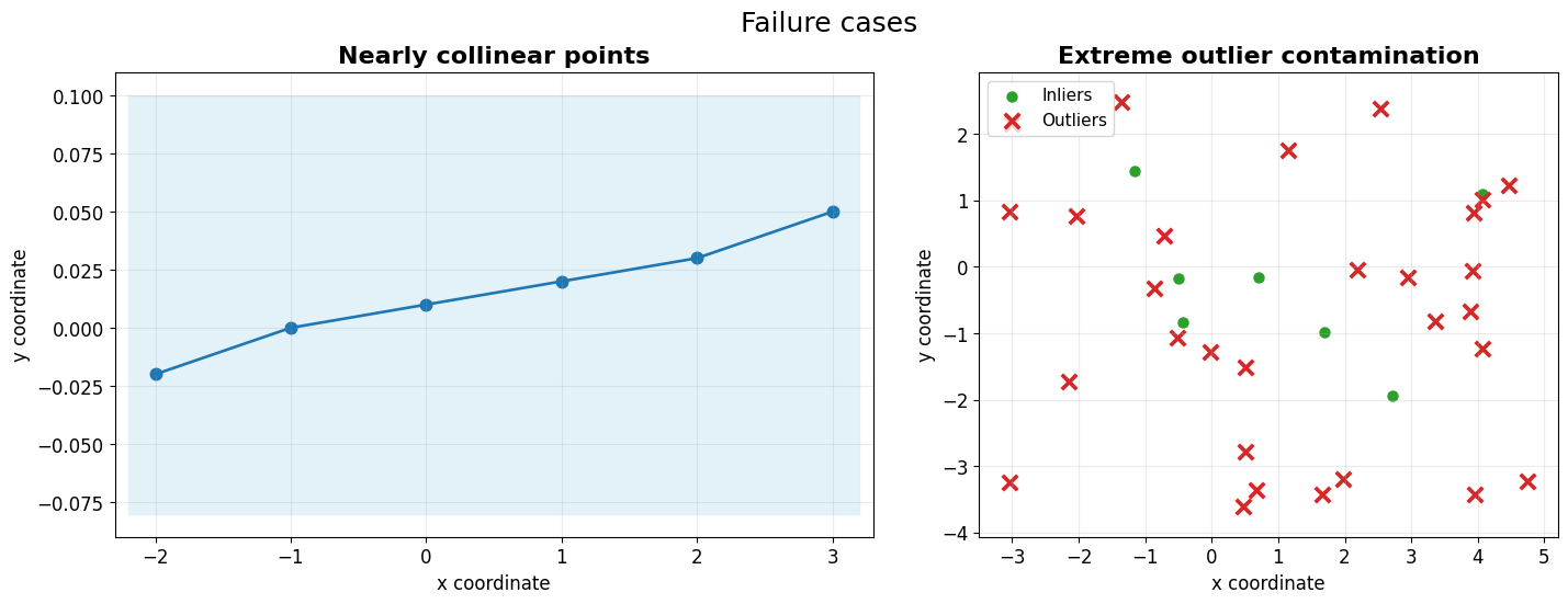
Homography estimation needs well-conditioned correspondences. Two common problems are:

Nearly collinear points: the DLT system is poorly constrained because the points do not span the plane.
Too many outliers: RANSAC may never draw a minimal sample made only of inliers.

The left panel shows a narrow band of nearly collinear points; the right shows a field dominated by outliers with only a few inliers. A low error on a thin strip of points does not mean the homography is stable over the whole plane, and overwhelming outliers can defeat even a robust estimator. Good estimation needs both clean matches and good spatial coverage.

collinear_src = torch.tensor(
    [
        [-2.0, -0.02],
        [-1.0,  0.00],
        [ 0.0,  0.01],
        [ 1.0,  0.02],
        [ 2.0,  0.03],
        [ 3.0,  0.05],
    ]
)
collinear_dst = apply_homography(collinear_src, H_gt)
collinear_dst = collinear_dst + 0.01 * torch.randn_like(collinear_dst)

H_collinear = estimate_homography_dlt(collinear_src, collinear_dst)
collinear_error = compute_reprojection_error(H_collinear, collinear_src, collinear_dst).mean().item()
collinear_matrix_error = torch.linalg.norm(normalize_homography_scale(H_collinear) - normalize_homography_scale(H_gt)).item()

src_hard, _, dst_hard, true_inliers_hard = generate_correspondences(H_gt, noise_std=0.08, outlier_ratio=0.80)
try:
    H_hard, hard_inliers, hard_info = ransac_homography(src_hard, dst_hard, threshold=0.20, num_iters=500)
    hard_matrix_error = torch.linalg.norm(normalize_homography_scale(H_hard) - normalize_homography_scale(H_gt)).item()
    hard_status = f"succeeded, matrix error={hard_matrix_error:.3f}, inlier ratio={hard_info['inlier_ratio']:.2f}"
except RuntimeError as exc:
    hard_status = f"failed: {exc}"

print("Nearly collinear case")
print("  Mean reprojection error:", collinear_error)
print("  Matrix error vs ground truth:", collinear_matrix_error)
print()
print("Extreme-outlier RANSAC case")
print(" ", hard_status)

Nearly collinear case
  Mean reprojection error: 0.012909880897369538
  Matrix error vs ground truth: 5.157270021755176

Extreme-outlier RANSAC case
  succeeded, matrix error=2.797, inlier ratio=0.19

Summary

You implemented, in PyTorch and from scratch:

homogeneous coordinate conversion,
point normalization,
normalized DLT,
reprojection error,
RANSAC-based robust fitting,
and inverse image warping for perspective correction.

The experiments showed that:

normalized DLT works well when correspondences are clean and well spread out,
RANSAC is essential when mismatches are present,
inverse warping turns an estimated homography into a dense rectification tool,
degenerate point sets and extreme outlier rates can still defeat the estimator.

A natural extension is to replace the synthetic corners with real detections and study how interpolation, occlusion, and imperfect corner localization affect rectification.

Found an error on this page? Report an issue.

Physical AI

3D Reconstruction

Imitation Learning

World Models

VLA Models

Sim-to-Real Transfer

Homographies and Robust Estimation

What a homography does

Homogeneous coordinates and $\tilde{\mathbf{p}}' \sim H\tilde{\mathbf{p}}$

Synthetic data setup

Visualizing the known transformation

Noisy correspondences and outliers

Estimation: DLT versus RANSAC

RANSAC inliers and outliers

Validation against ground truth

Perspective correction with inverse warping

Parameter study

Failure cases: degeneracy and extreme outliers

Summary

​What a homography does

​Homogeneous coordinates and p~′∼Hp~\tilde{\mathbf{p}}' \sim H\tilde{\mathbf{p}}p~​′∼Hp~​

​Synthetic data setup

​Visualizing the known transformation

​Noisy correspondences and outliers

​Estimation: DLT versus RANSAC

​RANSAC inliers and outliers

​Validation against ground truth

​Perspective correction with inverse warping

​Parameter study

​Failure cases: degeneracy and extreme outliers

​Summary

What a homography does

Homogeneous coordinates and $\tilde{\mathbf{p}}' \sim H\tilde{\mathbf{p}}$

Synthetic data setup

Visualizing the known transformation

Noisy correspondences and outliers

Estimation: DLT versus RANSAC

RANSAC inliers and outliers

Validation against ground truth

Perspective correction with inverse warping

Parameter study

Failure cases: degeneracy and extreme outliers

Summary